Electronic focusing II
In the previous modules we observed that, the ultrasound signal can be focused both on transmit and receive. Moreover, we observed that focusing benefits both lateral resolution and sensitivity. Now we will see how this translates into improved image quality. To simplify the coding, we will use the UltraSound ToolBox (www.ustb.no) which is being developed here at ISB.
Related material:
Alfonso Rodriguez-Molares <alfonso.r.molares@ntnu.no>
Stefano Fiorentini <stefano.fiorentini@ntnu.no>
Last edit 16-09-2020
Scanning again
Now that we have modelled array transducers and electronic focusing we should try to scan an image again. Now we don’t need to mechanically steer and move the transducer. Instead, we can perform a scan by properly activating different array elements each time.
We will model the L11 Verasonics probe. The L11 has 128 elements. To perform a scan, we can acquire the first scan line using the first 32 elements, the second scan line using elements from 2 to 33, the third scanline using elements from 3 to 34, and so on… As we proceed acquiring scan lines, we are filling the columns of a 2-D image. The focal point moves laterally with the active aperture, but keeping the same focal depth.
We are going to use the UltraSound Toolbox (USTB), which can be downloaded from the link above. Make sure USTB is installed and inside the MATLAB path before you continue.
The probe
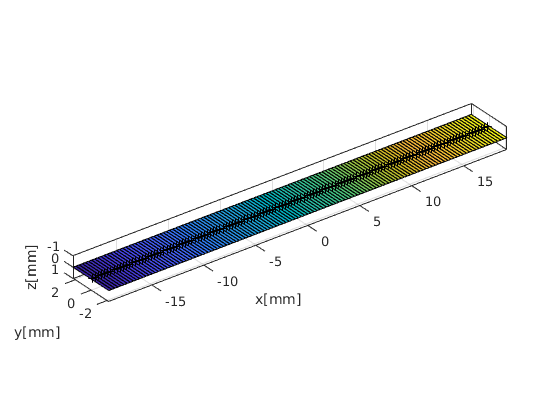
We start by defining the L11 transducer. The L11 is a 128 elements linear transducer with 300 um pitch. Each element is 270 um wide and 4.5 mm high
probe = uff.linear_array('N',128,...                % number elements
                         'pitch',300e-6,...         % pitch [m]
                         'element_width',270e-6,... % element width [m]
                         'element_height',4.5e-3);  % element height [m]
h = probe.plot();
The pulse
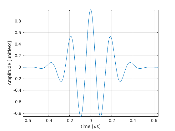
We need to define the ultrasound pulse that will be transmitted. Here we will use a pulse with 5.2 MHz center frequency and a 60% fractional bandwidth
pulse = uff.pulse('center_frequency', 5.2e6,...      % center frequency [Hz]
                  'fractional_bandwidth', 0.6);      % fractional bandwidth [unitless]
pulse.plot();
The phantom
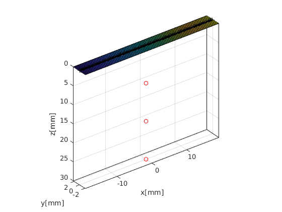
We define a phantom containing three scatterers centered at x = 0 mm, located at depths z = [10, 20, 30] mm, with scattering coefficient \(\Gamma=1\).
Gamma=1;
phantom = uff.phantom();
phantom.points =   [0, 0, 10e-3, Gamma;...
                    0, 0, 20e-3, Gamma;...
                    0, 0, 30e-3, Gamma];
phantom.plot(h);
The sequence
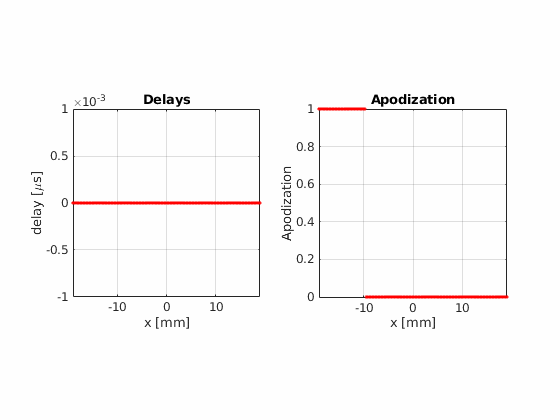
We define the beam profile that we will use in each of the transmit events. This is done by setting the delays and apodization values that will be used for each transmit event. In our case we want to use 32 elements at a time and shift the active aperture by one element at a time. That makes a total of 97 transmit events, or scan lines.
We start with unfocused beams. This means that we are not going to apply transmit delays.
N_active_elements=32;
N_scanlines=probe.N_elements-N_active_elements+1;
filename = 'unfocused_sequence.gif';
sequence = uff.wave();

h = figure('Color', 'w');
for n=1:N_scanlines
    active_elements = (1:32)+n-1;

    sequence(n) = uff.wave();
    sequence(n).probe = probe;
    sequence(n).sound_speed=1540;

    % apodization
    apodization = zeros(1,probe.N_elements);
    apodization(active_elements)=1;
    sequence(n).apodization = uff.apodization('apodization_vector',apodization);
    x_axis(n)=mean(probe.x(active_elements));

    % source
    sequence(n).source=uff.point('xyz', [x_axis(n), 0, -Inf]);

    sequence(n).plot(h);
    drawnow()

    % Capture the plot as an image
    frame = getframe(h);
    im = frame2im(frame);
    [imind,cm] = rgb2ind(im,256);

    % Write to the GIF File
    if n == 1
        imwrite(imind, cm, filename, 'gif' , 'Loopcount', inf, 'DelayTime', 0.1);
    else
        imwrite(imind, cm, filename, 'gif', 'WriteMode', 'append', 'DelayTime', 0.1);
    end
end
The Fresnel simulator
We integrated the Fresnel formulation into a compact simulator. We just have to input all the structures we defined so far and specify a sampling frequency. In this example we will set a 100 MHz sampling frequency.
sim=fresnel();

sim.phantom=phantom;            % phantom
sim.pulse=pulse;                % transmitted pulse
sim.probe=probe;                % probe
sim.sequence=sequence;          % beam sequence
sim.sampling_frequency=100e6;   % sampling frequency [Hz]

channel_data=sim.go();
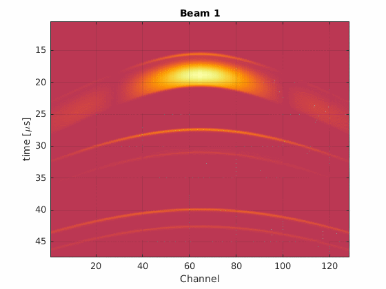
From the simulator we obtain RF (radio frequency) channel data, also referred to as raw data. This is the type of data obtained from an ultrasound scanner before any kind of processing. The next example will plot channel data for every transmit event, so you check how it looks.
h = figure('Color', 'w');
filename = 'unfocused_channel_data.gif';
for n=1:N_scanlines
    channel_data.plot(h, n);
    drawnow()

    % Capture the plot as an image
    frame = getframe(h);
    im = frame2im(frame);
    [imind,cm] = rgb2ind(im,256);

    % Write to the GIF File
    if n == 1
        imwrite(imind, cm, filename, 'gif', 'Loopcount', inf, 'DelayTime', 0.1);
    else
        imwrite(imind, cm, filename, 'gif', 'WriteMode', 'append', 'DelayTime', 0.1);
    end
end
Generating an image
To generate a scanline we just need to sum the receive signal from the active channels. A complete image is formed by all the scanlines. Don’t forget to transform the time axis into a depth axis.
for n=1:N_scanlines
    % we apply the same apodization function that we applied on transmit
    channel_data.data(:,:,n) = ...
        bsxfun(@times,channel_data.data(:,:,n),sequence(n).apodization.data.');
end

z_axis = channel_data.time*channel_data.sound_speed/2;
b_image = squeeze(sum(channel_data.data,2));
envelope = abs(hilbert(b_image));
envelope_dB = 20*log10(envelope/max(envelope(:)));

figure('color', 'w')
imagesc(x_axis*1e3,z_axis*1e3,envelope_dB)
axis equal tight
colormap gray
colorbar
caxis([-60 0])
xlabel('x [mm]')
ylabel('z [mm]')
title('Unfocused beams')
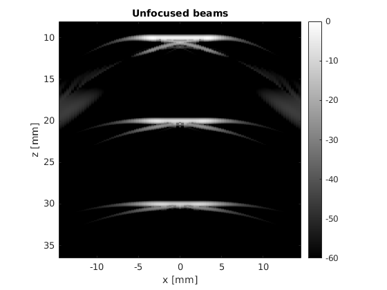
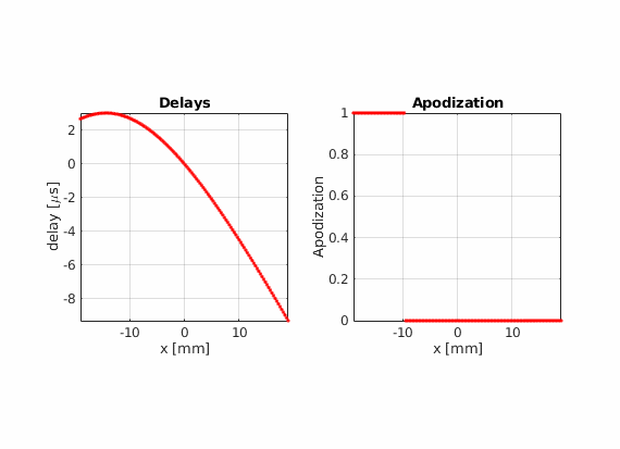
Focused beams
The result is not that good, but we can improve image quality by focusing the signal on transmit and on receive. We define a new sequence, in which the active elements are focused. The focal point is located in the middle of the active aperture and at 20 mm depth.
focal_depth=20e-3;
N_active_elements=32;
N_scanlines=probe.N_elements-N_active_elements+1;
filename = 'focused_sequence.gif';
sequence = uff.wave();

h = figure('Color', 'w');
for n=1:N_scanlines
    active_elements = (1:32)+n-1;

    sequence(n) = uff.wave();
    sequence(n).probe = probe;
    sequence(n).sound_speed=1540;

    % apodization
    apodization = zeros(1,probe.N_elements);
    apodization(active_elements)=1;
    sequence(n).apodization = uff.apodization('apodization_vector',apodization);
    x_axis(n)=mean(probe.x(active_elements));

    % source
    sequence(n).source=uff.point('xyz',[x_axis(n), 0, focal_depth]);

    % plot
    sequence(n).plot(h);

    % Capture the plot as an image
    frame = getframe(h);
    im = frame2im(frame);
    [imind,cm] = rgb2ind(im,256);

    % Write to the GIF File
    if n == 1
        imwrite(imind, cm, filename, 'gif', 'Loopcount', inf, 'DelayTime',0.1);
    else
        imwrite(imind, cm, filename, 'gif', 'WriteMode', 'append', 'DelayTime', 0.1);
    end
end
We launch the simulation again and we plot the simulated channel data.
h = figure('Color', 'w');
filename = 'focused_channel_data.gif';
for n=1:N_scanlines
    channel_data.plot(h,n);

    % Capture the plot as an image
    frame = getframe(h);
    im = frame2im(frame);
    [imind,cm] = rgb2ind(im,256);

    % Write to the GIF File
    if n == 1
        imwrite(imind, cm, filename, 'gif', 'Loopcount', inf, 'DelayTime', 0.1);
    else
        imwrite(imind, cm, filename, 'gif', 'WriteMode', 'append', 'DelayTime', 0.1);
    end
end

To focus on receive, we need to delay the signal received by each channel. To do so, we can use the same delay profiles used on transmit. Moreover, we can apply on the receive data the same apodization values that we used in transmit. Finally, we can sum the delayed receive data.
delayed_data=zeros(size(channel_data.data));
for n=1:N_scanlines

    % we apply the same apodization function that we applied on transmit
    channel_data.data(:,:,n) = ...
        bsxfun(@times,channel_data.data(:,:,n),sequence(n).apodization.data.');

    % delay-and-sum (DAS) takes place here
    for m=1:channel_data.N_channels
        delayed_data(:,m,n)=interp1(channel_data.time,channel_data.data(:,m,n),...
            channel_data.time-sequence(n).delay_values(m),'linear',0);
    end
end

z_axis = channel_data.time*channel_data.sound_speed/2;
b_image = squeeze(sum(delayed_data,2));
envelope = abs(hilbert(b_image));
envelope_dB = 20*log10(envelope/max(envelope(:)));

figure('Color', 'w');
imagesc(x_axis*1e3,z_axis*1e3,envelope_dB)
axis equal tight
grid on
box on
set(gca, 'Layer', 'top')
colormap gray
colorbar
caxis([-60 0])
xlabel('x [mm]')
ylabel('z [mm]')
title('Focused beams')
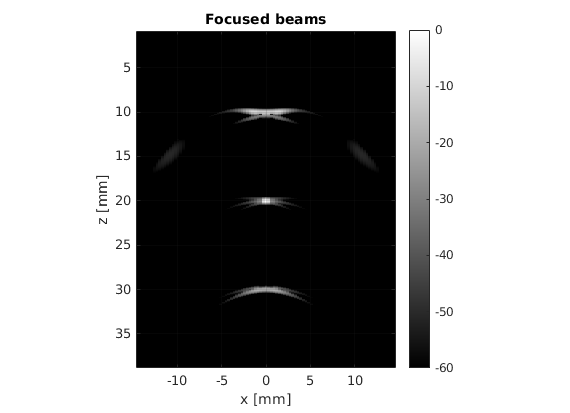
Why does the points at 20 mm look sharp, whereas the other two are smeared out?
Can you think of any way of solving this problem?