Electronic focusing I

Array transducers allow us to focus and steer whith greater flexibility compared to convex transducers. In this module we will learn about how we can operate an array of transducers to achieve electronic focusing.

Related material:

• Szabo Chapter 6

by Alfonso Rodriguez-Molares <alfonso.r.molares@ntnu.no>

updated by Stefano Fiorentini <stefano.fiorentini@ntnu.no>

Last edit 23-9-2020

One array element

Let us recall the Fraunhofer approximation for the signal back-scattered by a point reflector located at \(\vec{P} = (x_P, y_P, z_P)\), and received by a rectangular transducer located at \(\vec{T} = (x_T, y_T, z_T)\)

\[s_r(t, \vec{T}, \vec{P}) = \Gamma\frac{s(t-2r/c_{0})}{(4\pi r)^2}D^2(\theta, \phi)\]

where:

\begin{gather*} s(t) = \cos(2\pi f t)e^{-2.77(1.13t \Delta f)^2}\\ D(\theta, \phi) = \mathrm{sinc}\left(\frac{ka}{2\pi}\sin\theta\right)\mathrm{sinc}\left(\frac{kb}{2\pi}\sin\phi\right)\\ r = |\vec{P}-\vec{T}|\\ \theta = \arctan\left(\frac{x_P-x_T}{z_P-z_T}\right)\\ \phi = \arctan\left(\frac{y_P-y_T}{z_P-z_T}\right) \end{gather*}

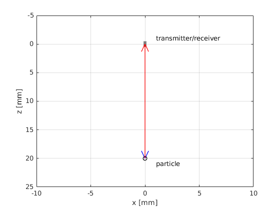
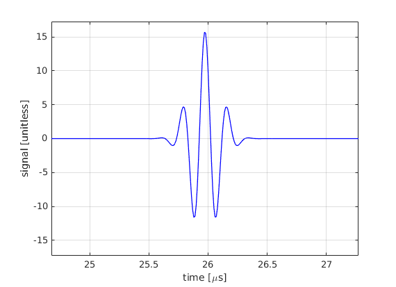
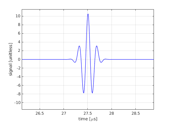
We are going to model a real array transducer, namely the L11 linear array from the Verasonics Vantage system. The array elements are 270 micrometers wide and 5 mm tall. The emitted pulse is Gaussian-shapped with 60% relative bandwidth bandwidth and 5.2 MHz center frequency. At the moment we will operate a single element of the array, which is centered at the origin of the coordinate system and is pointing downwards (positive z). Moreover, we will consider a single point scatterer located at \(\vec{P} = (0,0,20)\) mm with \(\Gamma=1\) reflection coefficient.

• Model and plot the received signal

frequency=5.2e6;                        % pulse frequency [MHz]
fractional_bandwidth=0.6;               % pulse fractional bandwidth [unitless]
Deltaf=fractional_bandwidth*frequency;  % pulse bandwidth [MHz]
c0=1540;                                % speed of sound [m/s]
lambda=c0/frequency;                    % wavelength [m]
k=2*pi*frequency/c0;                    % wavenumber [rad/m]
Fs=100e6;                               % sampling frequency [Hz]
time=0:(1/Fs):2*30e-3/c0;               % time vector [s]
width=270e-6;                           % element width [m]
height=5e-3;                            % element height [m]
Gamma=1;                                % reflection coefficient [unitless]

% geometrical variables
T=[0 0 0];                          % source-receiver position [m]
P=[0 0 20e-3];                      % point scatterer position [m]
theta=atan2(P(1)-T(1),P(3)-T(3));
phi=atan2(P(2)-T(2),P(3)-T(3));
distance=norm(T-P,2);

% the 2-way Fraunhofer model for rectangular elements
directivity = sinc(k*width/2.*sin(theta)/pi) .* ...
    sinc(k*height/2.*sin(phi)/pi);
received_signal=directivity.^2.*Gamma/(4*pi*distance)^2*...
cos(2*pi*frequency*(time-2*distance/c0)) .* ...
exp(-2.77*(1.1364*(time-2*distance/c0)*Deltaf).^2);

figure('Color', 'w')
rectangle('Position', [T(1)-width/2, T(3)-0.5e-3, width, 1e-3]*1e3, ...
    'FaceColor', [0.5, 0.5, 0.5], 'LineStyle', 'none')
hold on
text(T(1)*1e3 + 1, T(3)*1e3 - 1, 'transmitter/receiver');
quiver(T(1)*1e3, T(3)*1e3, (P(1)-T(1))*1e3, (P(3)-T(3))*1e3, 0, 'b', 'LineWidth', 1)
plot(P(1)*1e3, P(3)*1e3, 'ko', 'LineWidth', 1);
text(P(1)*1e3 + 1, P(3)*1e3 + 1, 'particle')
quiver(P(1)*1e3, P(3)*1e3, (T(1)-P(1))*1e3, (T(3)-P(3))*1e3, 0, 'r', 'LineWidth', 1)
box on 
grid on
xlabel('x [mm]');
ylabel('z [mm]');
xlim([-10, 10]);
ylim([-5, 25]);
set(gca, 'YDir', 'reverse');

figure('Color', 'w');
plot(time*1e6, received_signal, 'b', 'linewidth', 1);
box('on');grid on; axis tight;
xlabel('time [\mus]');
ylabel('signal [unitless]')
xlim(distance/c0*2*[0.95 1.05]*1e6);
ylim([-1.1*max(abs(received_signal)) 1.1*max(abs(received_signal))])

Two array elements

Let assume that we have two array elements, one placed at \(\vec{T} = (x_T, y_T, z_T)\) and the other placed at \(\vec{R} = (x_R, y_R, z_R)\). The point reflector is located at \(\vec{P} = (x_P, y_P, z_P)\) instead.

Can you derive the formula for the case when a pulse is sent from the element at \(\vec{P} = (-10,0,0)\) mm and received by the element at \(\vec{R} = (0,0,0)\) mm ?

• Model and plot the received signal

frequency=5.2e6;                        % pulse frequency [MHz]
fractional_bandwidth=0.6;               % pulse fractional bandwidth [unitless]
Deltaf=fractional_bandwidth*frequency;  % pulse bandwidth [MHz]
c0=1540;                                % speed of sound [m/s]
lambda=c0/frequency;                    % wavelength [m]
k=2*pi*frequency/c0;                    % wavenumber [rad/m]
Fs=100e6;                               % sampling frequency [Hz]
time=0:(1/Fs):2*30e-3/c0;               % time vector [s]
width=270e-6;                           % element width [m]
height=5e-3;                            % element height [m]
Gamma=1;                                % reflection coefficient [unitless]

% geometrical variables
T=[-10e-3, 0, 0];  % transmit element position [m]
R=[0, 0, 0];       % receiving element position [m]
P=[0, 0, 20e-3];   % point scatter position [m]

% transmitter part
theta_transmitter=atan2(P(1)-T(1),P(3)-T(3));
phi_transmitter=atan2(P(2)-T(2),P(3)-T(3));
distance_transmitter=norm(T-P,2);
directivity_transmitter = sinc(k*width/2.*sin(theta_transmitter)/pi) .* ...
    sinc(k*height/2.* sin(phi_transmitter)/pi);

% receiver part
theta_receiver=atan2(P(1)-R(1),P(3)-R(3));
phi_receiver=atan2(P(2)-R(2),P(3)-R(3));
distance_receiver=norm(R-P,2);
directivity_receiver = sinc(k*width/2.*sin(theta_receiver) .* ...
    cos(phi_receiver)/pi) .* ...
    sinc(k*height/2.*sin(theta_receiver) .* sin(phi_receiver)/pi);

% the 2-way Fraunhofer model for rectangular elements
received_signal=Gamma*directivity_receiver./(4*pi*distance_receiver) .* ...
    directivity_transmitter./(4*pi*distance_transmitter) .* ...
    cos(2*pi*frequency*(time-(distance_transmitter+distance_receiver)/c0)) .* ...
    exp(-2.77*(1.1364*(time-(distance_receiver+distance_transmitter)/c0)*Deltaf).^2);

figure('Color', 'w')
rectangle('Position', [T(1)-width/2, T(3)-0.5e-3, width, 1e-3]*1e3, ...
    'FaceColor', [0.5, 0.5, 0.5], 'LineStyle', 'none')
text(T(1)*1e3 + 1, T(3)*1e3 - 1, 'transmitter');
hold on
quiver(T(1)*1e3, T(3)*1e3, (P(1)-T(1))*1e3, (P(3)-T(3))*1e3, 0, 'b', 'LineWidth', 1)
plot(P(1)*1e3, P(3)*1e3, 'ko', 'LineWidth', 1);
text(P(1)*1e3 + 1, P(3)*1e3 + 1, 'particle')
quiver(P(1)*1e3, P(3)*1e3, (P(1)-R(1))*1e3, (R(3)-P(3))*1e3, 0, 'r', 'LineWidth', 1)
rectangle('Position', [R(1)-width/2, R(3)-0.5e-3, width, 1e-3]*1e3, ...
    'FaceColor', [0.5, 0.5, 0.5], 'LineStyle', 'none')
text(R(1)*1e3 + 1, R(3)*1e3 - 1, 'receiver');
box on 
grid on
xlabel('x [mm]');
ylabel('z [mm]');
xlim([-15, 5]);
ylim([-5, 25]);
set(gca, 'YDir', 'reverse');

figure('Color', 'w');
plot(time*1e6,received_signal, 'b', 'linewidth',1);
box('on'); grid on; axis tight;
xlabel('time [\mus]');
ylabel('signal [unitless]')
xlim((distance_receiver+distance_transmitter)/c0*[0.95 1.05]*1e6);
ylim([-1.1*max(abs(received_signal)) 1.1*max(abs(received_signal))])

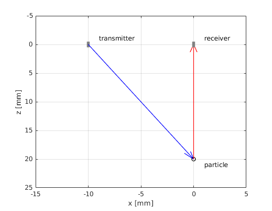
• Why has the signal reached the receive element at a later time, even though the point has not moved?

Transmit focusing

Now that we can model the wave propagation from any element to any other we are ready to introduce electronic focussing.

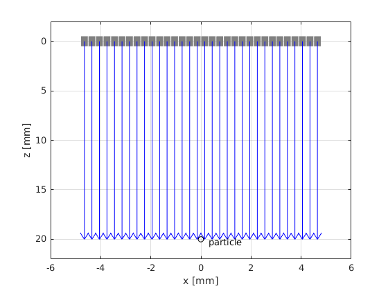
Let us consider an array of 32 elements. The distance between the center of consecutive elements is called pitch. The array pitch in the L11 transducer is 0.3 mm or 300 μm. The array is centered at the origin of the coordinate system, so that the center of the first element of the array is set at (-4.65, 0, 0) mm. Note that the array pitch is larger than the element width due to the manufacturing process of ceramic arrays. The gap between consecutive elements is called kerf.

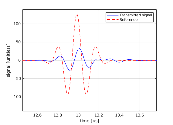
The transmitted pulse is obtained by adding the contribution of the 32 elements.

\[s_t(t, \vec{T}) = \sum_T \frac{s(t-r_T/c_0)}{4 \pi r_T} D^2(\theta_T, \phi_T)\]

• Plot the transmitted pulse obtained from 32 elements without transmit focusing. Compare it with the pulse that we would obtain if we operated a single element with 32 times higher voltage

frequency=5.2e6;                        % pulse frequency [MHz]
fractional_bandwidth=0.6;               % pulse fractional bandwidth [unitless]
Deltaf=fractional_bandwidth*frequency;  % pulse bandwidth [MHz]
c0=1540;                                % speed of sound [m/s]
lambda=c0/frequency;                    % wavelength [m]
k=2*pi*frequency/c0;                    % wavenumber [rad/m]
Fs=100e6;                               % sampling frequency [Hz]
time=0:(1/Fs):2*30e-3/c0;               % time vector [s]
width=270e-6;                           % element width [m]
height=5e-3;                            % element height [m]
N_elements=32;                          % number of elements
pitch=300e-6;                           % array pitch

Gamma=1;                                % reflection coefficient [unitless]

x0=((1:N_elements)*pitch);
x0=x0-mean(x0);
geom=[x0.', zeros([N_elements, 2])];

% phantom variables
P=[0, 0, 20e-3];                   % point scatter position [m]

% transmitter part
theta_transmitter=atan2(P(1)-geom(:,1),P(3)-geom(:,3));
phi_transmitter=atan2(P(2)-geom(:,2),P(3)-geom(:,3));
distance_transmitter=sqrt(sum((geom-ones(N_elements,1)*P).^2,2));
directivity_transmitter = sinc(k*width/2.*sin(theta_transmitter) .* ...
    cos(phi_transmitter)/pi).* ...
    sinc(k*height/2.*sin(theta_transmitter) .* sin(phi_transmitter)/pi);

% Fraunhofer model for rectangular elements
transmitted_signal=zeros(size(time));

for n=1:N_elements
    transmitted_signal = transmitted_signal+directivity_transmitter(n) ./ ...
        (4*pi*distance_transmitter(n))*...
        cos(2*pi*frequency*(time-distance_transmitter(n)/c0)) .* ...
        exp(-2.77*(1.1364*(time-distance_transmitter(n)/c0)*Deltaf).^2);
end

reference_signal = 32./(4*pi*P(3))*cos(2*pi*frequency*(time-P(3)/c0)) .*...
    exp(-2.77*(1.1364*(time-P(3)/c0)*Deltaf).^2);

figure('Color', 'w')
hold on
for i = 1:size(geom, 1)
    rectangle('Position', [geom(i,1)-width/2, geom(i,3)-0.5e-3, width, 1e-3]*1e3, ...
        'FaceColor', [0.5, 0.5, 0.5], 'LineStyle', 'none')
end
quiver(geom(:,1)*1e3, geom(:,3)*1e3,(P(1)*ones([size(geom, 1), 1]))*1e3, ...
    (P(3)-geom(:,3))*1e3, 0, 'b', 'MaxHeadSize', 0.1)
plot(P(1)*1e3,P(3)*1e3,'ko')
text(P(1)*1e3+0.3,P(3)*1e3+0.3,'particle')
grid on
box on
xlabel('x [mm]')
ylabel('z [mm]')
xlim([-6, 6])
ylim([-2, 22])
set(gca, 'YDir', 'reverse')


figure('Color', 'w')
plot(time*1e6,transmitted_signal,'b','linewidth',1)
hold on
plot(time*1e6,reference_signal,'r--','linewidth',1)
xlabel('time [\mus]')
ylabel('signal [unitless]')
xlim(mean(distance_transmitter)/c0*[0.95 1.05]*1e6)
legend('Transmitted signal','Reference')
ylim([-1.1*max(abs(reference_signal)), 1.1*max(abs(reference_signal))])
box on
grid on

We can focus the ultrasound beam on transfmit by activating the elements of the array with a time delay. The goal is to ensure that each emitted pulse reaches the focus at the same time.

\begin{gather*} s_t(t, \vec{T}) = \sum_T \frac{s(t-r_T/c_0 - \delta_T)}{4 \pi r_T} D^2(\theta_T, \phi_T)\\ \delta_T = \frac{|\vec{F}|- |\vec{T}-\vec{F}|}{c_0} \end{gather*}

where \(\delta_T\) denotes the transmit focus delay and \(\vec{F} = (x_F, y_F, z_F)\) denotes the focal point.

• Set the focus to (0, 0, 20) mm. Plot the transmitted pulse and compare it with the signal that we would obtain if we operated a single element with 32 times higher voltage

frequency=5.2e6;                        % pulse frequency [MHz]
fractional_bandwidth=0.6;               % pulse fractional bandwidth [unitless]
Deltaf=fractional_bandwidth*frequency;  % pulse bandwidth [MHz]
c0=1540;                                % speed of sound [m/s]
lambda=c0/frequency;                    % wavelength [m]
k=2*pi*frequency/c0;                    % wavenumber [rad/m]
Fs=100e6;                               % sampling frequency [Hz]
time=0:(1/Fs):2*30e-3/c0;               % time vector [s]
width=270e-6;                           % element width [m]
height=5e-3;                            % element height [m]
N_elements=32;                          % number of elements
pitch=300e-6;                           % array pitch

Gamma=1;                                % reflection coefficient [unitless]

x0=((1:N_elements)*pitch);
x0=x0-mean(x0);
geom=[x0.', zeros([N_elements, 2])];

% geometrical variables
P=[0 0 20e-3];                       % point scatter position [m]
focus=[0 0 20e-3];                   % focus position [m]

% transmitter part
theta_transmitter=atan2(P(1)-geom(:,1),P(3)-geom(:,3));
phi_transmitter=atan2(P(2)-geom(:,2),P(3)-geom(:,3));
distance_transmitter=sqrt(sum((geom-ones(N_elements,1)*P).^2,2));
directivity_transmitter = sinc(k*width/2.*sin(theta_transmitter)/pi).*...
    sinc(k*height/2*sin(phi_transmitter)/pi);
focusing_delay=(norm(focus,2)-sqrt(sum((geom-ones(N_elements,1)*focus).^2,2)))/c0;

% Fraunhofer model for rectangular elements
transmitted_signal=zeros(size(time));
for n=1:N_elements
    transmitted_signal = transmitted_signal+directivity_transmitter(n) ./ ...
        (4*pi*distance_transmitter(n)) .* ...
        cos(2*pi*frequency*(time-distance_transmitter(n)/c0-focusing_delay(n))) .* ...
        exp(-2.77*(1.1364*(time-distance_transmitter(n)/c0-focusing_delay(n))*Deltaf).^2);
end
reference_signal=32./(4*pi*P(3))*cos(2*pi*frequency*(time-P(3)/c0)).*...
    exp(-2.77*(1.1364*(time-P(3)/c0)*Deltaf).^2);

figure('Color', 'w')
hold on
for i = 1:size(geom, 1)
    rectangle('Position', [geom(i,1)-width/2, geom(i,3)-0.5e-3, width, 1e-3]*1e3, ...
        'FaceColor', [0.5, 0.5, 0.5], 'LineStyle', 'none')
end
quiver(geom(:,1)*1e3, geom(:,3)*1e3,(P(1)-geom(:,1))*1e3, (P(3)-geom(:,3))*1e3, ...
    0, 'b', 'MaxHeadSize', 0.1)
plot(P(1)*1e3,P(3)*1e3,'ko')
text(P(1)*1e3+0.3,P(3)*1e3+0.3,'particle')
grid on
box on
xlabel('x [mm]')
ylabel('z [mm]')
xlim([-6, 6])
ylim([-2, 22])
set(gca, 'YDir', 'reverse')

figure('Color', 'w')
plot(time*1e6,transmitted_signal,'b','linewidth',1)
box on
grid on
axis tight
hold on
plot(time*1e6,reference_signal,'r--','linewidth',1)
xlabel('time [\mus]')
ylabel('signal [unitless]')
xlim(mean(distance_transmitter)/c0*[0.95 1.05]*1e6)
legend('Transmitted signal','Reference')
ylim([-1.1*max(abs(reference_signal)) 1.1*max(abs(reference_signal))])

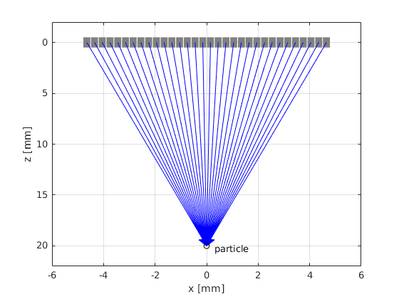
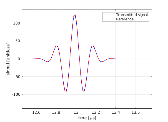
• Why is there a difference in the amplitude between the focused and unfocused case?

Receive focusing

We can focus the receive signal in a similar fashion

\begin{gather*} s_r(t, \vec{R}) = \sum_R \frac{s(t-r_R/c_0 - \delta_R)}{4 \pi r_R} D^2(\theta_R, \phi_R)\\ \delta_R = \frac{|\vec{F}|- |\vec{R}-\vec{F}|}{c_0} \end{gather*}

where \(\delta_R\) denotes the receive focus delay. It is possible to choose a different focal point on transmit \(\vec{F_T}\) and on receive \(\vec{F_R}\) but for practical reasons we will assume \(\vec{F} = \vec{F_T} = \vec{F_R}\).

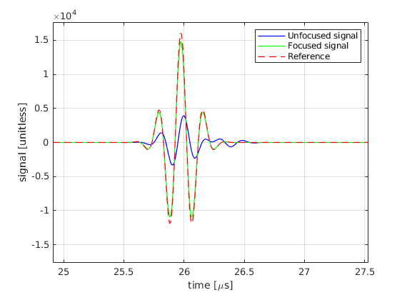
• Use the transmitted signal computed in the previous section and propagate it back to the transducer elements to model the receive data. Extract the receive signal samples at the correct time delay using interp1(). Compare the receive signal without receive focus and when the focus is set to (0,0,20) mm. Plot the signal that we would obtain if operated a single element with 1024 times higher voltage

frequency=5.2e6;                        % pulse frequency [MHz]
fractional_bandwidth=0.6;               % pulse fractional bandwidth [unitless]
Deltaf=fractional_bandwidth*frequency;  % pulse bandwidth [MHz]
c0=1540;                                % speed of sound [m/s]
lambda=c0/frequency;                    % wavelength [m]
k=2*pi*frequency/c0;                    % wavenumber [rad/m]
Fs=100e6;                               % sampling frequency [Hz]
time=0:(1/Fs):2*30e-3/c0;               % time vector [s]
width=270e-6;                           % element width [m]
height=5e-3;                            % element height [m]
N_elements=32;                          % number of elements
pitch=300e-6;                           % array pitch

Gamma=1;                                % reflection coefficient [unitless]

x0=((1:N_elements)*pitch);
x0=x0-mean(x0);
geom=[x0.', zeros([N_elements, 2])];

% geometrical variables
P=[0 0 20e-3];                       % point scatter position [m]
focus=[0 0 20e-3];                   % focus position [m]

% transmitter part
theta_transmitter=atan2(P(1)-geom(:,1),P(3)-geom(:,3));
phi_transmitter=atan2(P(2)-geom(:,2),P(3)-geom(:,3));
distance_transmitter=sqrt(sum((geom-ones(N_elements,1)*P).^2,2));
directivity_transmitter = sinc(k*width/2.*sin(theta_transmitter)/pi).*...
    sinc(k*height/2.*sin(phi_transmitter)/pi);
focusing_delay=(norm(focus,2)-sqrt(sum((geom-ones(N_elements,1)*focus).^2,2)))/c0;

% Fraunhofer model for rectangular elements
transmitted_signal=zeros(size(time));
for n=1:N_elements
    transmitted_signal = transmitted_signal+directivity_transmitter(n) ./ ...
        (4*pi*distance_transmitter(n)) .* ...
        cos(2*pi*frequency*(time-distance_transmitter(n)/c0-focusing_delay(n))) .* ...
        exp(-2.77*(1.1364*(time-distance_transmitter(n)/c0-focusing_delay(n))*Deltaf).^2);
end

% receiver part
theta_receiver=atan2(P(1)-geom(:,1),P(3)-geom(:,3));
phi_receiver=atan2(P(2)-geom(:,2),P(3)-geom(:,3));
distance_receiver=sqrt(sum((geom-ones(N_elements,1)*P).^2,2));
directivity_receiver = sinc(k*width/2.*sin(theta_transmitter) .* ...
    cos(phi_transmitter)/pi).*...
sinc(k*height/2.*sin(theta_transmitter).*sin(phi_transmitter)/pi);
focusing_delay=(norm(focus,2)-sqrt(sum((geom-ones(N_elements,1)*focus).^2,2)))/c0;

% Fraunhofer model for rectangular elements
received_signal_unfocused=zeros(size(time));
received_signal_focused=zeros(size(time));
for n=1:N_elements
    % unfocused signal
    delayed_signal=interp1(time,transmitted_signal,time - ...
        distance_receiver(n)/c0);
    received_signal_unfocused = received_signal_unfocused + ...
        directivity_receiver(n)./...
    (4*pi*distance_receiver(n)) .* delayed_signal;
    % focused signal
    delayed_signal=interp1(time,transmitted_signal,time - ...
        distance_receiver(n)/c0-focusing_delay(n));
    received_signal_focused=received_signal_focused + ...
        directivity_receiver(n)./...
    (4*pi*distance_receiver(n)).*delayed_signal;
end

reference_signal=1024./(4*pi*P(3))^2*cos(2*pi*frequency*(time-2*P(3)/c0)).*...
exp(-2.77*(1.1364*(time-2*P(3)/c0)*Deltaf).^2);

figure('Color', 'w')
plot(time*1e6,received_signal_unfocused,'b','linewidth',1)
hold on
plot(time*1e6,received_signal_focused,'g','linewidth',1)
plot(time*1e6,reference_signal,'r--','linewidth',1)
xlabel('time [\mus]')
ylabel('signal [unitless]')
xlim(2*mean(distance_transmitter)/c0*[0.95 ,1.05]*1e6)
legend('Unfocused signal','Focused signal','Reference')
ylim([-1.1*max(abs(reference_signal)), 1.1*max(abs(reference_signal))])
box on
grid on