Focusing and Steering
This section is about how to model focusing and steering using the knowledge developed in the Physics module. We will then use these concepts to investigate how transducer parameters such as size and frequency affect image quality.
Related material:
Alfonso Rodriguez-Molares <alfonso.r.molares@ntnu.no>
Stefano Fiorentini <stefano.fiorentini@ntnu.no>
Last edit 15-09-2020
Simple cardiac probe
A simple cardiac probe consists of a single element transducer mounted on a motor. A line of sight is reconstructed by sending an ultrasound pulse and recording the back-scattered echoes. Once the acquisition is complete, the motor changes the orientation of the transducer by a small angle so that a new line of sight can be acquired. The procedure is repeated until the entire field of view is covered. In the next example we are going to simulate the image of an object acquired with this setup. Lets assume we have a 20 mm x 5 mm rectangular transducer. The transducer emits a pulse with 3.25 MHz center frequency.
% Transducer properties
f0 = 3.25e6;                          % pulse frequency [MHz]
df = 0.6*f0;                          % pulse bandwidth [MHz]
c0 = 1540;                            % speed of sound [m/s]
lambda = c0/f0;                       % wavelength [m]
k = 2*pi*f0/c0;                       % wavenumber [rad/m]
Fs = 100e6;                           % sampling frequency [Hz]
a = 20e-3;                            % transducer width [m]
b = 5e-3;                             % transducer height [m]
s = [0, 0 ,0];                        % transducer position [m]

% Imaging variables
t = 0:(1/Fs):2*70e-3/c0;                  % time vector [s]
range = t*c0/2;                           % range vector [m]
azimuth = linspace(-pi/4, pi/4, 256);     % azimuth vector [rad]

% Phantom
Gamma=1;                            % reflection coefficient [unitless]
p =      [0, 0, 20e-3; ...          % collection of point scatterers
    0, 0, 30e-3; ...
    0, 0, 40e-3; ...
    0, 0, 50e-3; ...
    0, 0, 60e-3; ...
    -20e-3, 0, 40e-3; ...
    20e-3, 0, 40e-3];

% Scanning
im = zeros([length(azimuth), length(range)]);

for i = 1:length(azimuth)

    for j = 1:length(p)
        theta = atan2(p(j,1)-s(1),p(j,3)-s(3))-azimuth(i);
        phi = atan2(p(j,2)-s(2),p(j,3)-s(3));
        distance = sqrt(sum((s-p(j,:)).^2));

        % 2-way Fraunhofer model for rectangular elements
        directivity = abs(sinc(k*a/2.*sin(theta)/pi) .* ...
            sinc(k*b/2.*sin(phi)/pi));

        im(i, :) = im(i,:) + directivity.^2 .* Gamma./(4*pi*distance).^2 .* ...
            cos(2*pi*f0*(t-2*range/c0)) .* ...
            exp(-2.77*(1.1364*(t-2*distance/c0)*df).^2);
    end
end

% convert to intensity values
env = abs(hilbert(im))+eps;
env_dB = 20*log10(env./max(env(:)));

% plot
[AZ, R] = ndgrid(azimuth, range);
[Z, X] = pol2cart(AZ, R);

figure('Color', 'w');
colormap gray
surface(X*1e3, Z*1e3, env_dB, 'LineStyle', 'none')
axis tight equal;
box on
grid on
set(gca, 'Layer', 'top', 'YDir', 'reverse')
xlabel('x [mm]')
ylabel('z [mm]')
caxis([-60 0])
colorbar
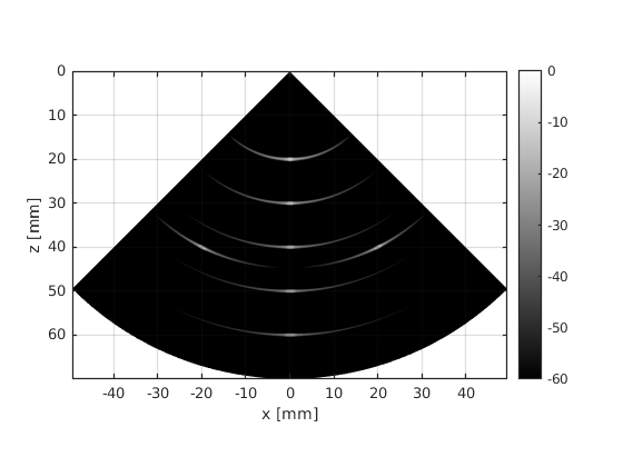
The result is not impressive. The lateral resolution in the image is rather poor. Morever, the objects exhibit a high sidelobe level. But we are on our way to solve that.
Pressure field of a flat transducer
For starters, let’s recall the Rayleigh integral that we introduced in the Physics section:
where \(\vec{r} = (x_{r}, y_{r}, z_{r})\) is point in which the pressure field is evaluated, \(\vec{s} = (x_{s}, y_{s}, z_{s})\) is a point on the radiating surface, \(r = |\vec{r}-\vec{s}|\) is the distance, \(v_{0}\) [m/s] is the surface velocity and \(\omega\) [rad/s] is the excitation angular frequency.
Lets assume we have a 20 mm x 5 mm rectangular transducer. The transducer oscillates at 3.25 MHz and with 1e-3 m/s surface velocity. The transducer is centered at the origin of the coordinate stystem and is surrounded by a medium with 1540 m/s sound speed and 1020 kg/m3 density. One way to numerically solve the integral is to use a Monte-Carlo approach. However, in order to get accurate results, a high number of sources is needed.
We are going to define a grid of points that satisfies \(az \in [-\pi/4, pi/4]\) rad and \(z \in [1, 70]\) mm. Represent the beam pattern with a dynamic range of 40 dB.
% Transducer properties
f0 = 3.25e6;                          % pulse frequency [MHz]
df = 0.6*f0;                          % pulse bandwidth [MHz]
c0 = 1540;                            % speed of sound [m/s]
lambda = c0/f0;                       % wavelength [m]
w0 = 2*pi*f0;                         % angular frequency [rad/s]
k = w0/c0;                            % wavenumber [rad/m]
a = 20e-3;                            % transducer width [m]
b = 5e-3;                             % transducer height [m]

rho = 1020;                           % fluid density [kg/m3]
v0 = 1e-3;                            % surface velocity [m/s]

% Simulation parameters
N = 1e5;
chunksize = 5e3;
N_chunks = N / chunksize;

az = linspace(-pi/4, pi/4, 256);
r = linspace(0, 7e-2, 256);
[AZ, R] = ndgrid(az, r);
[Z, X] = pol2cart(AZ, R);

N_pixels = numel(X);

map = zeros(1, N_pixels);                         % map we want to create

for n = 1:N_chunks
    fprintf(1, 'Computing chunk %d of %d\n', n, N_chunks);

    % We set random source location within the transducer surface
    s = [random('unif',-a/2, a/2,chunksize,1), ...
        random('unif',-b/2, b/2,chunksize,1), ...
        zeros(chunksize,1)];

    % Compute distance from all sources to all pixels
    R = sqrt(   (s(:,1) - X(:).').^2 + ...
                s(:,2).^2 + ...
                Z(:).^2.');

    % Compute Green function
    green = exp(-1i*k*R)./(2*pi*R);

    % We add the contribution from all sources
    map =  map + sum(green);
end

% Calculate pressure field
map = 1j*w0*rho*v0*map;

% Reshape results;
map = reshape(map, size(X));

% Apply log compression
map = 20*log10(abs(map) / max(abs(map(:))));

% Plot
figure('Color', 'w')
surface(X*1e3, Z*1e3, map, 'LineStyle', 'none')
box on
grid on;
set(gca, 'YDir', 'reverse', 'Layer', 'top')
colorbar
caxis([-40 0])
axis equal tight
xlabel('x [mm]')
ylabel('z [mm]')
title('SPL [dB]')
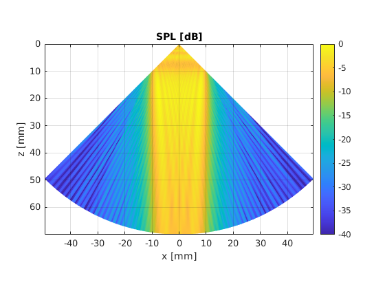
A major cause of degraded image quality in the first picture is caused by the excessive width of the ultrasound beam.
Focusing
We will now modify the transducer to focus at 40 mm depth. In practice, this can be achieved by manufacturing curved transducers, by placing an acoustic lens in front of the transducer, or using array transducers (more on this later).
Mathematically this is equivalent to inserting the following phase term in the Rayleigh integral
where \(\vec{f}=(x_{f}, y_{f}, z_{f})\) is the focal point and \(k = \frac{\omega}{c_{0}}\) [rad/m] is the wave number.
Set the focal point at \(\vec{f} = (0, 0, 20)\) mm. Calculate the phase factor, include it in the Rayleigh integral and check the effect on the beam profile.
% Transducer properties
f0 = 3.25e6;                            % pulse frequency [MHz]
df = 0.6*f0;                            % pulse bandwidth [MHz]
c0 = 1540;                              % speed of sound [m/s]
lambda = c0/f0;                         % wavelength [m]
w0 = 2*pi*f0;                           % angular frequency [rad/s]
k = w0/c0;                              % wavenumber [rad/m]
a = 20e-3;                              % transducer width [m]
b = 5e-3;                               % transducer height [m]
focus = [0, 0, 4e-2];                   % focus position [m]
rho = 1020;                             % fluid density [kg/m3]
v0 = 1e-3;                              % surface velocity [m/s]


% Simulation parameters
N = 1e5;
chunksize = 5e3;
N_chunks = N / chunksize;

az = linspace(-pi/4, pi/4, 256);
r = linspace(0, 7e-2, 256);
[AZ, R] = ndgrid(az, r);
[Z, X] = pol2cart(AZ, R);

N_pixels = numel(X);

map = zeros(1, N_pixels);                         % map we want to create

for n = 1:N_chunks
    fprintf(1, 'Computing chunk %d of %d\n', n, N_chunks);

    % We set random source location within the transducer surface
    s = [random('unif',-a/2, a/2,chunksize,1), ...
        random('unif',-b/2, b/2,chunksize,1), ...
        zeros(chunksize,1)];

    % Compute distance from all sources to all pixels
    R = sqrt(   (s(:,1) - X(:).').^2 + ...
                s(:,2).^2 + ...
                Z(:).^2.');

    % Compute the focusing distance difference
    Rf = sqrt(sum((s-focus).^2, 2))-sqrt(sum(focus.^2));

    % Compute Green function
    green = exp(1i*k*Rf) .* exp(-1i*k*R)./(2*pi*R);

    % We add the contribution from all sources
    map =  map + sum(green);
end

% Calculate pressure field
map = 1j*w0*rho*v0*map;

% Reshape results;
map = reshape(map, size(X));

% Apply log compression
map = 20*log10(abs(map) / max(abs(map(:))));

% Plot
figure('Color', 'w')
surface(X*1e3, Z*1e3, map, 'LineStyle', 'none')
box on
grid on;
set(gca, 'YDir', 'reverse', 'Layer', 'top')
colorbar
caxis([-40 0])
axis equal tight
xlabel('x [mm]')
ylabel('z [mm]')
title('SPL [dB]')
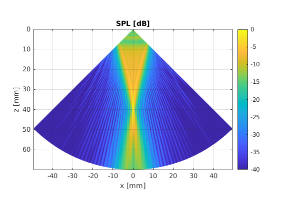
By focusing the ultrasound beam we greatly reduce the ultrasound beam width. This will result in improved lateral resolution in the final image.
Steering
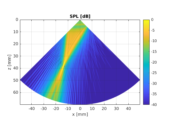
The beam can also be steered in a similar fashion.
Check out the beam profile when it is steered by \(\theta = -20\) degrees.
% Transducer properties
f0 = 3.25e6;                            % transducer frequency [MHz]
df = 0.6*f0;                            % pulse bandwidth [MHz]
c0 = 1540;                              % speed of sound [m/s]
lambda = c0/f0;                         % wavelength [m]
w0 = 2*pi*f0;                           % angular frequency [rad/s]
k = w0/c0;                              % wavenumber [rad/m]
a = 20e-3;                              % element width [m]
b = 5e-3;                               % element height [m]
focus = [sind(-20), 0, cosd(-20)]*4e-2; % Focus position [m]
rho = 1020;                             % Fluid density [kg/m3]
v0 = 1e-3;                              % Surface velocity [m/s]


% Simulation parameters
N = 1e5;
chunksize = 5e3;
N_chunks = N / chunksize;

az = linspace(-pi/4, pi/4, 256);
r = linspace(0, 7e-2, 256);
[AZ, R] = ndgrid(az, r);
[Z, X] = pol2cart(AZ, R);

N_pixels = numel(X);

map = zeros(1, N_pixels);                         % map we want to create

for n = 1:N_chunks
    fprintf(1, 'Computing chunk %d of %d\n', n, N_chunks);

    % We set random source location within the transducer surface
    s = [random('unif',-a/2, a/2,chunksize,1), ...
        random('unif',-b/2, b/2,chunksize,1), ...
        zeros(chunksize,1)];

    % Compute distance from all sources to all pixels
    R = sqrt(   (s(:,1) - X(:).').^2 + ...
                s(:,2).^2 + ...
                Z(:).^2.');

    % Compute the focusing distance difference
    Rf = sqrt(sum((s-focus).^2, 2))-sqrt(sum(focus.^2));

    % Compute Green function
    green = exp(1i*k*Rf) .* exp(-1i*k*R)./(2*pi*R);

    % We add the contribution from all sources
    map =  map + sum(green);
end

% Calculate pressure field
map = 1j*w0*rho*v0*map;

% Reshape results;
map = reshape(map, size(X));

% Apply log compression
map = 20*log10(abs(map) / max(abs(map(:))));

% Plot
figure('Color', 'w')
surface(X*1e3, Z*1e3, map, 'LineStyle', 'none')
box on
grid on;
set(gca, 'YDir', 'reverse', 'Layer', 'top')
colorbar
caxis([-40 0])
axis equal tight
xlabel('x [mm]')
ylabel('z [mm]')
title('SPL [dB]')
The influence of transducer size, frequency, and focal depth
Using the same approach we can also appreciate how pulse frequency, transducer size and focal depth affect the width of the ultrasound beam. For convenience, we are going to look at a the beam profile at the focal depth only.
Set the transducer width to 1cm, 2cm, 3cm and 4cm. Plot the lateral beam profile at the focal depth.
% Transducer properties
f0 = 3.25e6;                            % pulse frequency [MHz]
df = 0.6*f0;                            % pulse bandwidth [MHz]
c0 = 1540;                              % speed of sound [m/s]
lambda = c0/f0;                         % wavelength [m]
w0 = 2*pi*f0;                           % angular frequency [rad/s]
k = w0/c0;                              % wavenumber [rad/m]
a = [1e-2, 2e-2, 3e-3, 4e-2];           % transducer width [m]
b = 5e-3;                               % transducer height [m]
focus = [0, 0, 4e-2];                   % focus position [m]
rho = 1020;                             % fluid density [kg/m3]
v0 = 1e-3;                              % surface velocity [m/s]


% Simulation parameters
N = 1e5;
chunksize = 5e3;
N_chunks = N / chunksize;

x = linspace(-2.5e-3, 2.5e-3, 256);
z = focus(3);

map = zeros(length(a), 256);                % map we want to create

for i = 1:length(a)
    for n = 1:N_chunks
        fprintf(1, 'Computing chunk %d of %d\n', n, N_chunks);

        % We set random source location within the transducer surface
        s = [random('unif',-a(i)/2, a(i)/2, chunksize,1), ...
            random('unif',-b/2, b/2, chunksize,1), ...
            zeros(chunksize,1)];

        % Compute distance from all sources to all pixels
        R = sqrt((s(:,1) - x).^2 + ...
            s(:,2).^2 + ...
            z.^2);

        % Compute the focusing distance difference
        Rf = sqrt(sum((s-focus).^2, 2))-sqrt(sum(focus.^2));

        % Compute Green function
        green = exp(1i*k*Rf) .* exp(-1i*k*R)./(2*pi*R);

        % We add the contribution from all sources
        map(i, :) = map(i, :) + sum(green);
    end
end
% Calculate pressure field
map = 1j*w0*rho*v0*map;

% Apply log compression
map = 20*log10(abs(map) ./ max(abs(map), [], 2));

% Plot
figure('Color', 'w')
plot(x*1e3, map, 'LineWidth', 1)
box on
grid on;
set(gca, 'Layer', 'top')
axis tight
xlabel('x [mm]')
ylabel('SPL [dB]')
ylim([-20, 0])
legend({'a = 10mm', 'a = 20mm', 'a = 30mm', 'a = 40mm'})
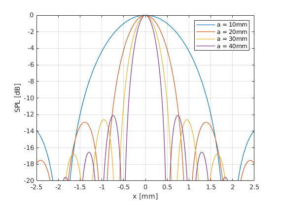
We can see that the beam width is inversely proportional to the transducer size. Therefore, large transducers lead to improved lateral resolution. Unfortunately this is not possible in every application (i.e. intercostal space in cardiac imaging defines a upper boundary to the transducer size). Now let’s check the influence of imaging depth.
Set the transducer width back to 2cm, and set focal depth to 1cm, 2cm, 3cm and 4cm. Plot the lateral beam profile at the focal depth.
% Transducer properties
f0 = 3.25e6;                            % pulse frequency [MHz]
df = 0.6*f0;                            % pulse bandwidth [MHz]
c0 = 1540;                              % speed of sound [m/s]
lambda = c0/f0;                         % wavelength [m]
w0 = 2*pi*f0;                           % angular frequency [rad/s]
k = w0/c0;                              % wavenumber [rad/m]
a = 2e-2;                               % transducer width [m]
b = 5e-3;                               % transducer height [m]
focus = [0, 0, 1e-2; ...
        0, 0, 2e-2; ...
        0, 0, 3e-2; ...
        0, 0, 4e-2];                   % focus position [m]
rho = 1020;                             % fluid density [kg/m3]
v0 = 1e-3;                              % surface velocity [m/s]


% Simulation parameters
N = 1e5;
chunksize = 5e3;
N_chunks = N / chunksize;

x = linspace(-2.5e-3, 2.5e-3, 256);

map = zeros(size(focus, 1), 256);                % map we want to create

for i = 1:size(focus, 1)
    z = focus(i, 3);

    for n = 1:N_chunks
        fprintf(1, 'Computing chunk %d of %d\n', n, N_chunks);

        % We set random source location within the transducer surface
        s = [random('unif',-a/2, a/2, chunksize,1), ...
            random('unif',-b/2, b/2, chunksize,1), ...
            zeros(chunksize,1)];

        % Compute distance from all sources to all pixels
        R = sqrt((s(:,1) - x).^2 + ...
            s(:,2).^2 + ...
            z.^2);

        % Compute the focusing distance difference
        Rf = sqrt(sum((s-focus(i, :)).^2, 2))-sqrt(sum(focus(i, :).^2));

        % Compute Green function
        green = exp(1i*k*Rf) .* exp(-1i*k*R)./(2*pi*R);

        % We add the contribution from all sources
        map(i, :) = map(i, :) + sum(green);
    end
end
% Calculate pressure field
map = 1j*w0*rho*v0*map;

% Apply log compression
map = 20*log10(abs(map) ./ max(abs(map), [], 2));

% Plot
figure('Color', 'w')
plot(x*1e3, map, 'LineWidth', 1)
box on
grid on;
set(gca, 'Layer', 'top')
axis tight
xlabel('x [mm]')
ylabel('SPL [dB]')
ylim([-20, 0])
legend({'z = 1cm', 'z = 2cm', 'z = 3cm', 'z = 4cm'})
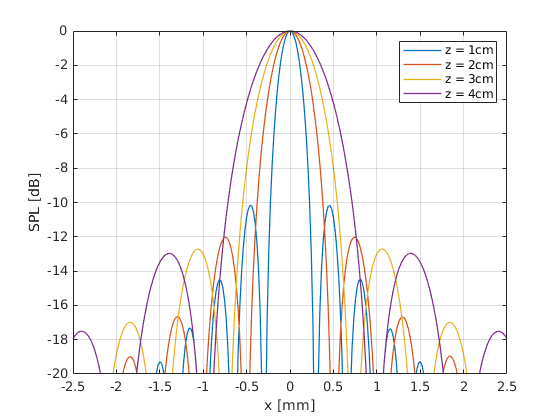
We can see that, given a fixed transducer width, the ultrasound beam becomes wider as the focal depth increases. Therefore, lateral resolution degrades with imaging depth. Finally, let’s check the influence of pulse frequency.
Set the the focal depth back to 4cm, and set the pulse frequency to 3.25 MHz, 4.25 MHz, 5.25 MHz and 6.25 MHz. Plot the lateral beam profile at the focal depth.
% Transducer properties
f0 = [3.25e6, 4.25e6, 5.25e6, 6.25e6];  % pulse frequency [MHz]
df = 0.6*f0;                            % pulse bandwidth [MHz]
c0 = 1540;                              % speed of sound [m/s]
lambda = c0./f0;                         % wavelength [m]
w0 = 2*pi*f0;                           % angular frequency [rad/s]
k = w0/c0;                              % wavenumber [rad/m]
a = 2e-2;                               % transducer width [m]
b = 5e-3;                               % transducer height [m]
focus = [0, 0, 4e-2];                   % focus position [m]
rho = 1020;                             % fluid density [kg/m3]
v0 = 1e-3;                              % surface velocity [m/s]


% Simulation parameters
N = 1e5;
chunksize = 5e3;
N_chunks = N / chunksize;

x = linspace(-2.5e-3, 2.5e-3, 256);
z = focus(3);

map = zeros(length(f0), 256);                % map we want to create

for i = 1:length(f0)
    for n = 1:N_chunks
        fprintf(1, 'Computing chunk %d of %d\n', n, N_chunks);

        % We set random source location within the transducer surface
        s = [random('unif',-a/2, a/2, chunksize,1), ...
            random('unif',-b/2, b/2, chunksize,1), ...
            zeros(chunksize,1)];

        % Compute distance from all sources to all pixels
        R = sqrt((s(:,1) - x).^2 + ...
            s(:,2).^2 + ...
            z.^2);

        % Compute the focusing distance difference
        Rf = sqrt(sum((s-focus).^2, 2))-sqrt(sum(focus.^2));

        % Compute Green function
        green = exp(1j*k(i)*Rf) .* exp(-1j*k(i)*R)./(2*pi*R);

        % We add the contribution from all sources
        map(i, :) = map(i, :) + sum(green);
    end
    % Calculate pressure field
    map(i, :) = 1j*w0(i)*rho*v0*map(i, :);
end

% Apply log compression
map = 20*log10(abs(map) ./ max(abs(map), [], 2));

% Plot
figure('Color', 'w')
plot(x*1e3, map, 'LineWidth', 1)
box on
grid on;
set(gca, 'Layer', 'top')
axis tight
xlabel('x [mm]')
ylabel('SPL [dB]')
ylim([-20, 0])
legend({'f0 = 3.25MHz', 'f0 = 4.25MHz', 'f0 = 5.25MHz', 'f0 = 6.25MHz'})
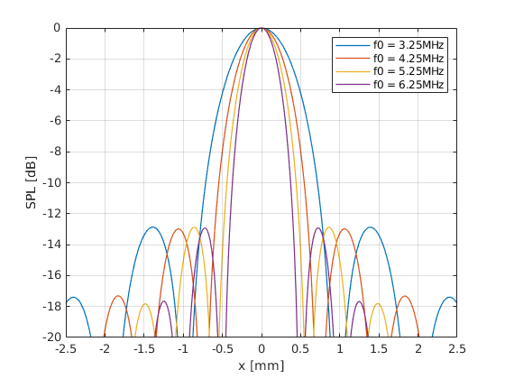
We can see that the beam width is inversely proportional to the pulse frequency. High pulse frequencies lead to improved lateral resolution (we have already seen in the Physics section that high pulse frequencies lead to improved axial resolution). However, remember that high frequencies are attenuated faster. Therefore, high frequencies are not an option if high imaging depth are needed. One case is cardiac imaging.
Sre you able to derive the same conclusions by looking at the Fraunhofer aproximation of the beam profile for a rectangular transducer?