Multi Focus Imaging (MFI) and Dynamic Receive Focusing (DRF)
In this exercise we will explore a technique that is possible in electronically focused arrays to greatly improve the imaging quality.
Related material:
Alfonso Rodriguez-Molares <alfonso.r.molares@ntnu.no>
Stefano Fiorentini <stefano.fiorentini@ntnu.no>
Last edit 17-09-2020
Multi Focus Imaging (MFI)
We learned in the previous modules that focusing can be used to increase the signal intensity at a given depth and to improve the image lateral resolution. However, by chosing to focus at one depth we obtain an unfocused image elsewhere.
Wouldn’t it be nice to be able to focus everywhere?
One straightforward way of solving this challenge is to acquire multiple ultrasound images, each one with a different transmit focus depth, and to combine them. This technique is called Multi Focus Imaging (MFI) and has been used in commercial scanners until quite recently. We are going to expand the last example from the previous module to appreciate the difference.
Again, we are going to model a L11 Verasonics transducer. The array has 128 elements, 270 um wide and 4.5 mm tall. The array pitch is 300 um. The transmit pulse is gaussian shaped with 5.2 MHz center frequency and 60% relative bandwidth. We assume the array to be centered at the origin of the coordinate system. We are going to perform three acquisitions, with transmit focal depth set to 10mm, 20 mm and 30 mm, respectively. The active aperture used in each transmit event consists of 32 elements.
% probe
probe = uff.linear_array('N',128,...                % number elements
    'pitch',300e-6,...                              % pitch [m]
    'element_width',270e-6,...                      % element width [m]
    'element_height',4.5e-3);                       % element height [m]
N_active_elements = 32;
N_scanlines = probe.N_elements-N_active_elements+1;

% pulse
pulse = uff.pulse('center_frequency', 5.2e6,...     % center frequency [Hz]
    'fractional_bandwidth', 0.6);                   % fractional bandwidth [unitless]

% phantom
Gamma = 1;                                          % reflection coefficient [unitless]
phantom = uff.phantom();
phantom.points =   [     0,  0, 10e-3, Gamma;
    0,  0, 15e-3, Gamma;
    0,  0, 20e-3, Gamma;
    0,  0, 25e-3, Gamma;
    0,  0, 30e-3, Gamma;
    0,  0, 35e-3, Gamma];

% sequence
focal_depth = [10e-3, 20e-3, 30e-3];

sequence = uff.wave();
for f = 1:length(focal_depth)
    for n = 1:N_scanlines
        active_elements = (1:32)+n-1;

        sequence(f, n) = uff.wave();
        sequence(f, n).probe = probe;
        sequence(f, n).sound_speed=1540;            % speed of sound [m/s]

        % apodization
        apodization = zeros(1,probe.N_elements);
        apodization(active_elements)=1;
        sequence(f, n).apodization = uff.apodization('apodization_vector', apodization);
        x_axis(n) = mean(probe.x(active_elements));

        % source
        sequence(f, n).source=uff.point('xyz', [x_axis(n), 0, focal_depth(f)]);
    end
end

% generate channel_data
channel_data = uff.channel_data();
for f = 1:length(focal_depth)
    sim=fresnel();
    sim.phantom=phantom;                            % phantom
    sim.pulse=pulse;                                % transmitted pulse
    sim.probe=probe;                                % probe
    sim.sequence=sequence(f,:);                     % beam sequence
    sim.sampling_frequency=100e6;                   % sampling frequency [Hz]
    channel_data(f)=sim.go();
end

% beamforming
z_axis = 0:sequence(1).sound_speed/2/channel_data(1).sampling_frequency:40e-3;
beamformed_data = zeros([length(z_axis), length(x_axis), length(focal_depth)]);

h = waitbar(0, 'Beamforming');
for f = 1:length(focal_depth)
    for n=1:N_scanlines
        waitbar(n/N_scanlines, h);

        % we apply the same apodization function that we applied on transmit
        channel_data(f).data(:,:,n) = ...
            bsxfun(@times, channel_data(f).data(:,:,n), sequence(f,n).apodization.data.');

        delayed_data = zeros([length(z_axis), channel_data(f).N_channels]);

        % delay
        for m=1:channel_data(f).N_channels
            delayed_data(:,m)=interp1(channel_data(f).time,channel_data(f).data(:,m,n),...
                z_axis*2/sequence(f, n).sound_speed-sequence(f,n).delay_values(m), ...
                'linear',0);
        end

        % sum
        beamformed_data(:,n,f) = sum(delayed_data, 2);
    end
end
close(h)

% envelope extraction
beamformed_envelope = abs(hilbert(beamformed_data));

% plot single frames
figure('Color', 'w')
colormap gray
for f=1:length(focal_depth)
subplot(1,3,f)
imagesc(x_axis*1e3, z_axis*1e3, 20*log10(beamformed_envelope(:,:,f) / ...
    max(beamformed_envelope(:,:,f), [], 'all')))
axis equal tight
xlabel('x [mm]')
ylabel('z [mm]')
box on
grid on
set(gca, 'Layer', 'top')
caxis([-40,0])
colorbar
end

% MFI
mfi_data = sum(beamformed_data, 3);
mfi_envelope = abs(hilbert(mfi_data));

% plot MFI
figure('Color', 'w')
colormap gray
imagesc(x_axis*1e3, z_axis*1e3, 20*log10(mfi_envelope/max(mfi_envelope, [], 'all')))
axis equal tight
xlabel('x [mm]')
ylabel('z [mm]')
box on
grid on
set(gca, 'Layer', 'top')
caxis([-40,0])
colorbar
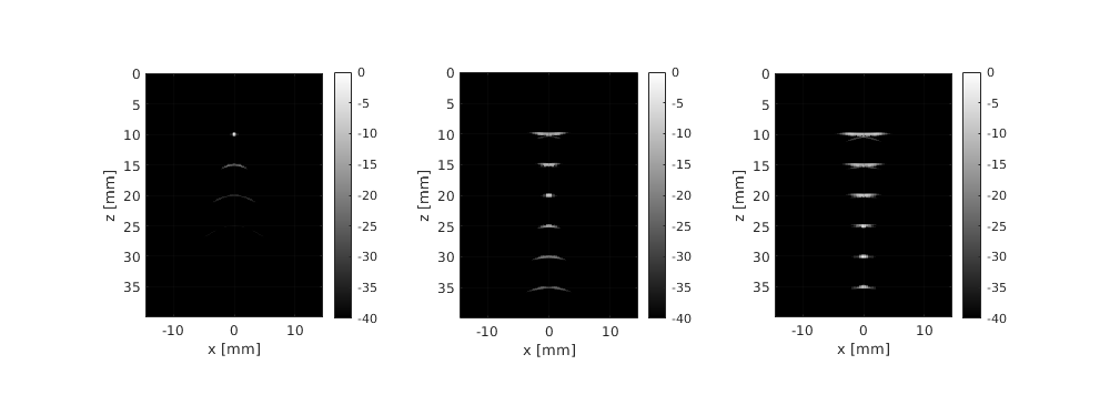
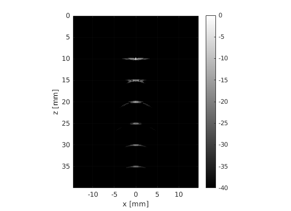
You can notice that the MFI image achieves a more uniform lateral resolution across the field of view. A downside of MFI is the reduced imaging framerate, since we need to acquire multiple images to make a single MFI image. Let us assume that we want to produce an image with 97 beams. Due to safety issues the pulse repetition frequency (PRF), which regulated the interval between consecutive transmit events, is limited to 5000 Hz.
Can you calculate the framerate in case 1, 2 and 3 focusing zones are used?
number_beams=97;        % number of beams
PRF=5000;               % pulse repetition frequency [Hz]
MFZ=[1, 2, 3];          % multifocal zones
framerate=PRF./(MFZ*number_beams);
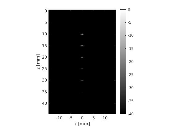
Dynamic Receive Focusing (DRF)
Luckily, there are other ways of improving image quality without affecting the framerate.
The transmit ultrasound beam cannot be focused everywhere. In fact, once a transmit delay profile is set and the transducer elements fire an ultrasound pulse, there is no way of changing the transmit focus position without having to fire a new pulse. On the other hand, we are free to interpolate channel data using an arbitrary number of receive delay profiles. This enables us to move the receive focus to every pixel in the image. This is Dynamic Receive Focusing (DRF) in a nutshell.
Let us consider the same scenario as in the previous exercise. This time we are going to set the transmit focal depth to 20 mm. We are also going to calculate and apply a different receive delay profile for every pixel in the image during the delay-and-sum (DAS) phase.
% probe
probe = uff.linear_array('N',128,...                % number elements
    'pitch',300e-6,...                              % pitch [m]
    'element_width',270e-6,...                      % element width [m]
    'element_height',4.5e-3);                       % element height [m]
N_active_elements = 32;
N_scanlines = probe.N_elements-N_active_elements+1;

% pulse
pulse = uff.pulse('center_frequency', 5.2e6,...     % center frequency [Hz]
    'fractional_bandwidth', 0.6);                   % fractional bandwidth [unitless]

% phantom
Gamma = 1;                                          % reflection coefficient [unitless]
phantom = uff.phantom();
phantom.points =   [     0,  0, 10e-3, Gamma;
    0,  0, 15e-3, Gamma;
    0,  0, 20e-3, Gamma;
    0,  0, 25e-3, Gamma;
    0,  0, 30e-3, Gamma;
    0,  0, 35e-3, Gamma];

% sequence
focal_depth = 10e-3;

sequence = uff.wave();
for n = 1:N_scanlines
    active_elements = (1:32)+n-1;

    sequence(n) = uff.wave();
    sequence(n).probe = probe;
    sequence(n).sound_speed=1540;               % speed of sound [m/s]

    % apodization
    apodization = zeros(1,probe.N_elements);
    apodization(active_elements)=1;
    sequence(n).apodization = uff.apodization('apodization_vector', apodization);
    x_axis(n) = mean(probe.x(active_elements));

    % source
    sequence(n).source=uff.point('xyz', [x_axis(n), 0, focal_depth]);
end

% generate channel_data
sim=fresnel();
sim.phantom=phantom;                            % phantom
sim.pulse=pulse;                                % transmitted pulse
sim.probe=probe;                                % probe
sim.sequence=sequence(f,:);                     % beam sequence
sim.sampling_frequency=100e6;                   % sampling frequency [Hz]
channel_data=sim.go();

% delay-and-sum (DAS) beamforming
delayed_data=zeros(size(channel_data.data));

z_axis = channel_data.time*channel_data.sound_speed/2;

h = waitbar(0, 'Beamforming');
for n=1:N_scanlines
    waitbar(n/N_scanlines, h);

    % we apply the same apodization function that we applied on transmit
    channel_data.data(:,:,n) = ...
        bsxfun(@times, channel_data.data(:,:,n), sequence(n).apodization.data.');

    for m=1:channel_data.N_channels

        % DRF
        distance=sqrt((probe.x(m)-x_axis(n)).^2+(probe.z(m)-z_axis).^2)-z_axis;
        delay=distance./channel_data.sound_speed;

        % delay
        delayed_data(:,m,n)=interp1(channel_data.time,channel_data.data(:,m,n),...
            channel_data.time+delay,'linear',0);
    end
end
close(h)

% sum
b_image = squeeze(sum(delayed_data,2));

% envelope extraction and log compression
envelope = abs(hilbert(b_image));
envelope_dB = 20*log10(envelope/max(envelope(:)));

% plot
figure('color', 'w')
imagesc(x_axis*1e3,z_axis*1e3,envelope_dB)
axis equal tight
colormap gray
colorbar
caxis([-40 0])
xlabel('x [mm]')
ylabel('z [mm]')
The only downside of DRF is the increased computational load. However, thanks to decades of gaming industry, we can purchase graphic cards that are able to crunch all these numbers in a jiffy. Moreover, DRF can be combined with MFI for even improved lateral resolution.
What effect does DRF have on the lateral resolution? And on the axial resolution?
Is the resolution improved at the transmit focal depth? Is anything improved a the focal depth?
How does DRF affect the framerate?
Is now the lateral resolution constant over the the whole field of view?