Apodization
In this module we will study what apodization is and how it can be implemented to improve image quality.
Related material:
Alfonso Rodriguez-Molares <alfonso.r.molares@ntnu.no>
Stefano Fiorentini <stefano.fiorentini@ntnu.no>
Last edit 18-09-2020
Apodization
The term apodization comes from the greek and can be translated to “removing the foot”. Apodization is used in several imaging applications to reduce diffraction patterns that occur around high intensity objects, and share many similarities with the windowing functions used in digital signal processing.
Until now we have been using a binary apodization function, i.e. we either used an element or we didn’t. Modern ultrasound scanners however, allow us to use arbitrary real-valued apodization functions, which can be used to further improve both the transmit and receive beam patterns. In the next examples, we will analyse how apodization can improve image quality.
One widely used apodization is the Hamming window:
where \(w_E\) is the weighting factor used for element \(E\), \(x_C\) is the center of the apodization window, \(x_E\) is the x coordinate of element \(E\), and \(L\) is the aperture size.
We consider the same scenario described in the Dynamic Receive Focusing (DRF) module. We model the L11 Verasonics probe. The array has 128 elements, 270 um wide and 5 mm tall. The array pitch is 300 um. The pulse is gaussian shaped with 5.2 MHz center frequency and 60% relative bandwidth. The array is centered at the origin of coordinates with its face pointing downwards (positive z). The transmit focal depth is 20 mm. Dynamic Receive Focusing is used. This time we are going to simulate a single point reflector with \(\Gamma=1\), located at \(P = (0, 0, 20)\) mm.
Beamform the image using 32 active elements and moving the aperture one element at a time.
% probe
probe = uff.linear_array('N',128,... % number elements
'pitch',300e-6,... % pitch [m]
'element_width',270e-6,... % element width [m]
'element_height',4.5e-3); % element height [m]
% pulse
pulse = uff.pulse('center_frequency', 5.2e6,... % pulse center frequency [Hz]
'fractional_bandwidth', 0.6); % pulse fractional bandwidth [unitless]
% phantom
Gamma=1;
phantom = uff.phantom();
phantom.points = [0, 0, 20e-3, Gamma];
% sequence
focal_depth=20e-3;
N_active_elements=32;
N_scanlines=probe.N_elements-N_active_elements+1;
sequence = uff.wave();
filename = 'flat_apodization.gif';
h = figure('Color', 'w');
for n=1:N_scanlines
active_elements = (1:32)+n-1;
sequence(n) = uff.wave();
sequence(n).probe = probe;
sequence(n).sound_speed=1540;
% apodization
apodization = zeros(1,probe.N_elements);
apodization(active_elements)=1; % binary apodization
sequence(n).apodization = uff.apodization('apodization_vector',apodization);
x_axis(n)=mean(probe.x(active_elements));
% source
sequence(n).source=uff.point('xyz',[x_axis(n) 0 focal_depth]);
% make animated gif
sequence(n).plot(h);
drawnow()
% Capture the plot as an image
frame = getframe(h);
im = frame2im(frame);
[imind,cm] = rgb2ind(im,256);
% Write to the GIF File
if n == 1
imwrite(imind,cm,filename,'gif', 'Loopcount',inf,'DelayTime',0.1);
else
imwrite(imind,cm,filename,'gif','WriteMode','append','DelayTime',0.1);
end
end
% simulation
sim=fresnel();
sim.phantom=phantom; % phantom
sim.pulse=pulse; % transmitted pulse
sim.probe=probe; % probe
sim.sequence=sequence; % beam sequence
sim.sampling_frequency=41.6e6; % sampling frequency [Hz]
channel_data=sim.go();
% delay-and-sum (DAS) beamforming
z_axis = channel_data.time*channel_data.sound_speed/2;
delayed_data=zeros(size(channel_data.data));
h = waitbar(0, 'Beamforming');
for n=1:N_scanlines
waitbar(n/N_scanlines, h);
% we apply the same apodization function that we applied on transmit
channel_data.data(:,:,n) = ...
bsxfun(@times, channel_data.data(:,:,n), sequence(n).apodization.data.');
for m=1:channel_data.N_channels
% DRF
distance=sqrt((probe.x(m)-x_axis(n)).^2+(probe.z(m)-z_axis).^2)-z_axis;
delay=distance./channel_data.sound_speed;
% delay
delayed_data(:,m,n)=interp1(channel_data.time,channel_data.data(:,m,n),...
channel_data.time+delay,'linear',0);
end
end
close(h)
% sum
b_image = squeeze(sum(delayed_data,2));
% envelope extraction
envelope = abs(hilbert(b_image));
% log compression
envelope_dB = 20*log10(envelope/max(envelope(:)));
figure('color', 'w');
imagesc(x_axis*1e3,z_axis*1e3,envelope_dB)
axis equal tight
colormap gray
colorbar
caxis([-60 0])
xlabel('x [mm]')
ylabel('z [mm]')
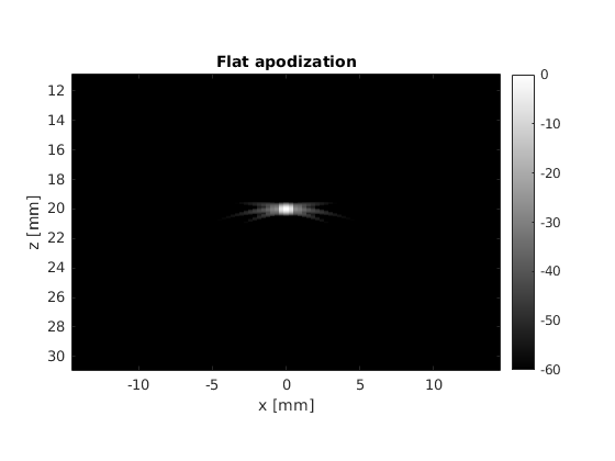
title('Flat apodization')
Now, using the same number of beams, beam positions and aperture size, try the hamming apodization both on transmit and on receive
% probe
probe = uff.linear_array('N',128,... % number elements
'pitch',300e-6,... % pitch [m]
'element_width',270e-6,... % element width [m]
'element_height',4.5e-3); % element height [m]
% pulse
pulse = uff.pulse('center_frequency', 5.2e6,... % pulse center frequency [Hz]
'fractional_bandwidth', 0.6); % pulse fractional bandwidth [unitless]
% phantom
Gamma=1;
phantom = uff.phantom();
phantom.points = [0, 0, 20e-3, Gamma];
% sequence
focal_depth=20e-3;
N_active_elements=32;
N_scanlines=probe.N_elements-N_active_elements+1;
sequence = uff.wave();
filename = 'hamming_apodization.gif';
h = figure('color', 'w');
for n=1:N_scanlines
active_elements = (1:32)+n-1;
sequence(n) = uff.wave();
sequence(n).probe = probe;
sequence(n).sound_speed=1540;
% apodization
apodization = zeros(1,probe.N_elements);
apodization(active_elements)=hamming(32); % hamming apodization
sequence(n).apodization = uff.apodization('apodization_vector',apodization);
x_axis(n)=mean(probe.x(active_elements));
% source
sequence(n).source=uff.point('xyz',[x_axis(n), 0, focal_depth]);
% make animated gif
sequence(n).plot(h);
drawnow;
% Capture the plot as an image
frame = getframe(h);
im = frame2im(frame);
[imind,cm] = rgb2ind(im,256);
% Write to the GIF File
if n == 1
imwrite(imind,cm,filename,'gif', 'Loopcount',inf,'DelayTime',0.1);
else
imwrite(imind,cm,filename,'gif','WriteMode','append','DelayTime',0.1);
end
end
% simulation
sim=fresnel();
sim.phantom=phantom; % phantom
sim.pulse=pulse; % transmitted pulse
sim.probe=probe; % probe
sim.sequence=sequence; % beam sequence
sim.sampling_frequency=41.6e6; % sampling frequency [Hz]
channel_data=sim.go();
% delay-and-sum (DAS) beamforming
z_axis = channel_data.time*channel_data.sound_speed/2;
delayed_data=zeros(size(channel_data.data));
h = waitbar(0, 'Beamforming');
for n=1:N_scanlines
waitbar(n/N_scanlines, h);
% we apply the same apodization function that we applied on transmit
channel_data.data(:,:,n) = ...
bsxfun(@times, channel_data.data(:,:,n), sequence(n).apodization.data.');
for m=1:channel_data.N_channels
% DRF
distance=sqrt((probe.x(m)-x_axis(n)).^2+(probe.z(m)-z_axis).^2)-z_axis;
delay=distance./channel_data.sound_speed;
% delay
delayed_data(:,m,n)=interp1(channel_data.time,channel_data.data(:,m,n),...
channel_data.time+delay,'linear',0);
end
end
close(h)
% sum
b_image = squeeze(sum(delayed_data,2));
% envelope extraction
envelope = abs(hilbert(b_image));
% log compression
envelope_dB = 20*log10(envelope/max(envelope(:)));
figure('color', 'w');
imagesc(x_axis*1e3,z_axis*1e3,envelope_dB)
axis equal tight
colormap gray
colorbar
caxis([-60 0])
xlabel('x [mm]')
ylabel('z [mm]')
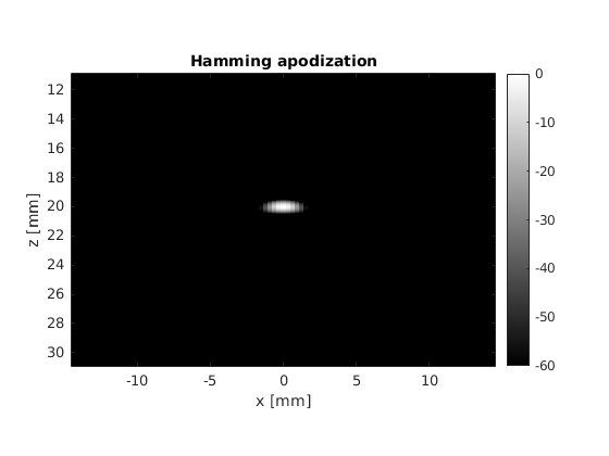
title('Hamming apodization')
Fraunhofer aproximation analysis
There are some clear differences between the two pictures, the most noticeable one being the suppression of the interference patterns around the main lobe. We can analyze this phenomenon in detail by leaveraging one of the properties of the Fraunhofer approximation.
At the focal depth, and for monochromatic pulses, the lateral profile of the PSF is equal to the Fourier transform of the apodization window. This means that we can estimate the lateral profile of the PSF by computing the FFT of the apodization window.
Compute a 1024-points FFT of both apodization windows (rectangular and hamming) for the central beam (n=48). Plot and compare the normalized amplitude of both FFTs.
% define the windows
% define the windows
n_beam=48;
rectangular_apodization=[zeros(1,n_beam-1), ones(1,N_active_elements),...
    zeros(1,probe.N_elements-(n_beam+N_active_elements)+1,1)].';
window_size=32;
hamming_apodization= zeros(1,probe.N_elements);
hamming_apodization((1:window_size)+n_beam-1)=hamming(window_size);

% compute the PSF as the FFT
rectangular_PSF=abs(fftshift(fft(rectangular_apodization,1024)));
    rectangular_PSF=rectangular_PSF./max(rectangular_PSF(:));
hamming_PSF=abs(fftshift(fft(hamming_apodization,1024)));
    hamming_PSF=hamming_PSF./max(hamming_PSF(:));

figure('Color','w')
subplot(2,1,1)
title('Apodization');
hold on
plot(rectangular_apodization, 'LineWidth', 1)
plot(hamming_apodization, 'LineWidth', 1)
box on
grid on
axis tight

subplot(2,1,2)
title('Lateral profile of PSF')
hold on
plot(20*log10(rectangular_PSF), 'LineWidth', 1)
plot(20*log10(hamming_PSF), 'LineWidth', 1)
grid on
box on
hold on
axis tight
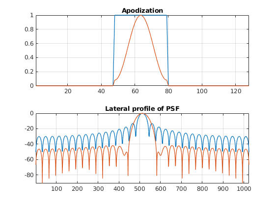
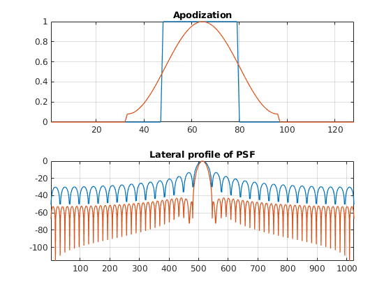
Can you see what is the point of hamming windows now? What has become better? What has become worse? How can you improve the lateral resolution of the hamming window
% define the windows
n_beam=48;
rectangular_apodization=[zeros(1,n_beam-1), ones(1,N_active_elements),...
    zeros(1,probe.N_elements-(n_beam+N_active_elements)+1,1)].';
window_size=64;
hamming_apodization= zeros(1,probe.N_elements);
hamming_apodization((1:window_size)+n_beam-16)=hamming(window_size);

% compute the PSF as the FFT
rectangular_PSF=abs(fftshift(fft(rectangular_apodization,1024)));
rectangular_PSF=rectangular_PSF./max(rectangular_PSF(:));
hamming_PSF=abs(fftshift(fft(hamming_apodization,1024)));
hamming_PSF=hamming_PSF./max(hamming_PSF(:));


figure('Color','w')
subplot(2,1,1)
title('Apodization');
hold on
plot(rectangular_apodization, 'LineWidth', 1)
plot(hamming_apodization, 'LineWidth', 1)
box on
grid on
axis tight

subplot(2,1,2)
title('Lateral profile of PSF')
hold on
plot(20*log10(rectangular_PSF), 'LineWidth', 1)
plot(20*log10(hamming_PSF), 'LineWidth', 1)
grid on
box on
hold on
axis tight
Towards pixel-based beamforming
There is another advantage of using real-valued apodizations. The beam center is no longer dependent on the array pitch. Therefore, the lateral distance between consecutive scan lines becomes arbitrary.
Using hamming apodization with an active aperture of L=19.2 mm, define a sequence composed of 256 beams where the beam center \(x_c\) goes from -14.4 mm to 14.4 mm.
% probe
probe = uff.linear_array('N',128,...                % number elements
                         'pitch',300e-6,...         % pitch [m]
                         'element_width',270e-6,... % element width [m]
                         'element_height',4.5e-3);  % element height [m]
% pulse
pulse = uff.pulse('center_frequency', 5.2e6,...     % pulse center frequency [Hz]
                  'fractional_bandwidth', 0.6);     % pulse fractional bandwidth [unitless]
% phantom
Gamma=1;
phantom = uff.phantom();
phantom.points =   [0,  0, 20e-3, Gamma];

% sequence
focal_depth=20e-3;
Active_aperture=19.2e-3;
N_scanlines=256;
x_axis=linspace(-14.4e-3,14.4e-3,N_scanlines);
sequence = uff.wave();
filename = 'interpolated_beams.gif';
h = figure('color', 'w');
for n=1:N_scanlines
    active_elements = (1:32)+n-1;

    sequence(n) = uff.wave();
    sequence(n).probe = probe;
    sequence(n).sound_speed=1540;

    % apodization
    xd=abs(probe.x-x_axis(n));                          % aperture distance [m]
    apodization = (double(xd<=Active_aperture/2).*...
    (0.5 + 0.5*cos(2*pi*xd./Active_aperture))).';       % hamming apodization
    sequence(n).apodization = uff.apodization('apodization_vector',apodization);

    % source
    sequence(n).source=uff.point('xyz',[x_axis(n), 0, focal_depth]);

    % make animated gif
    sequence(n).plot(h);
    drawnow;

    % Capture the plot as an image
    frame = getframe(h);
    im = frame2im(frame);
    [imind,cm] = rgb2ind(im,256);

    % Write to the GIF File
    if n == 1
        imwrite(imind, cm, filename, 'gif', 'Loopcount', inf, 'DelayTime', 0.1);
    else
        imwrite(imind, cm, filename, 'gif', 'WriteMode', 'append', 'DelayTime', 0.1);
    end
end

% simulation
sim=fresnel();
sim.phantom=phantom;            % phantom
sim.pulse=pulse;                % transmitted pulse
sim.probe=probe;                % probe
sim.sequence=sequence;          % beam sequence
sim.sampling_frequency=100e6;  % sampling frequency [Hz]
channel_data=sim.go();

% delay-and-sum (DAS) beamforming
z_axis = channel_data.time*channel_data.sound_speed/2;
delayed_data=zeros(size(channel_data.data));

h = waitbar(0, 'Beamforming');
for n=1:N_scanlines
    waitbar(n/N_scanlines, h);

    % we apply the same apodization function that we applied on transmit
    channel_data.data(:,:,n) = ...
        bsxfun(@times, channel_data.data(:,:,n), sequence(n).apodization.data.');

    for m=1:channel_data.N_channels
        % DRF
        distance=sqrt((probe.x(m)-x_axis(n)).^2+(probe.z(m)-z_axis).^2)-z_axis;
        delay=distance./channel_data.sound_speed;

        % delay
        delayed_data(:,m,n)=interp1(channel_data.time,channel_data.data(:,m,n),...
            channel_data.time+delay,'linear',0);
    end
end
close(h)

% sum
b_image = squeeze(sum(delayed_data,2));

% envelope extraction
envelope = abs(hilbert(b_image));

% log compression
envelope_dB = 20*log10(envelope/max(envelope(:)));

figure('color', 'w');
imagesc(x_axis*1e3,z_axis*1e3,envelope_dB)
axis equal tight
colormap gray
colorbar
caxis([-60 0])
xlabel('x [mm]')
ylabel('z [mm]')
title('Hamming apodization')

Modify the last example to move che point scatter towards the right or left side of the field of view. Does the PSF look the same compared to when it is placed in the center? Can you find an explanation for this?