Expanding Aperture
In this exercise we will study the effect of the aperture size on image quality and we will investigate a technique used in vascular imaging to achieve uniform lateral resolution in the field of view.
Related material:
Alfonso Rodriguez-Molares <alfonso.r.molares@ntnu.no>
Stefano Fiorentini <stefano.fiorentini@ntnu.no>
Last edit 21-09-2020
Aperture and lateral resolution
We have already noticed a few modules ago that there is a relation between aperture and lateral resolution. Let us study this quantitatively.
We consider the same scenario as in the apodization module. We are going to model the L11 Verasonics probe. The array has 128 elements, 270 um wide and 5 mm tall. The array pitch is 300 um. The emitted pulse is Gaussian-shaped with 5.2 MHz center frequency and 60% relative bandwidth. The array is centered at the origin of coordinate stystem. The focal points is located at 20 mm depth. Dynamic Receive Focusing (DRF) is used. A point reflector is placed at (0, 0, 20) mm. The scan consists of 96 beams, ranging from -2 mm to 2 mm on the x axis. Hamming apodization is used both on transmit and receive.
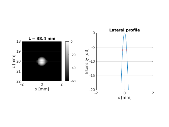
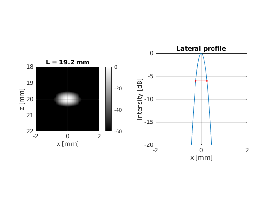
Set the active aperture to 38.4 mm, 19.2 mm, 9.6 mm, and 4.8 mm both on transmit and receive. For each case beamform the image and calculate the Full Width Half Maximum (FWHM) of the Point Spread Function (PSF) in the lateral direction.
% receive scan
N_scanlines=96;
x_axis=linspace(-2e-3, 2e-3, N_scanlines);

% probe
probe = uff.linear_array('N',128,...                % number elements
    'pitch',300e-6,...         % pitch [m]
    'element_width',270e-6,... % element width [m]
    'element_height',4.5e-3);  % element height [m]
% pulse
pulse = uff.pulse('center_frequency', 5.2e6,...     % center frequency [Hz]
    'fractional_bandwidth', 0.6);     % fractional bandwidth [unitless]
% phantom
Gamma=1;
phantom = uff.phantom();
phantom.points = [0,  0, 20e-3, Gamma];

% sequence
focal_depth = 20e-3;
L = [38.4e-3, 19.2e-3, 9.6e-3, 4.8e-3];             % Active aperture width
FWHM = zeros([1, length(L)]);

for i = 1:length(L)
    sequence = uff.wave();

    for n=1:N_scanlines
        % sequence definition
        sequence(n) = uff.wave();
        sequence(n).probe = probe;
        sequence(n).sound_speed=1540;

        % apodization
        xd=abs(probe.x-x_axis(n));            % aperture distance [m]
        apodization = (double(xd<=L(i)/2).*...
            (0.5 + 0.5*cos(2*pi*xd./L(i)))).';   % apodization
        sequence(n).apodization = uff.apodization('apodization_vector',apodization);

        % source
        sequence(n).source=uff.point('xyz', [x_axis(n), 0, focal_depth]);
    end

    % simulation
    sim=fresnel();
    sim.phantom=phantom;            % phantom
    sim.pulse=pulse;                % transmitted pulse
    sim.probe=probe;                % probe
    sim.sequence=sequence;          % beam sequence
    sim.sampling_frequency=100e6;   % sampling frequency [Hz]
    channel_data=sim.go();

    % delay-and-sum (DAS) beamforming
    z_axis = channel_data.time*channel_data.sound_speed/2;
    delayed_data=zeros(size(channel_data.data));

    h = waitbar(0, 'Beamforming');
    for n=1:N_scanlines
        waitbar(n/N_scanlines, h);

        % we apply the same apodization function that we applied on transmit
        channel_data.data(:,:,n) = ...
            bsxfun(@times, channel_data.data(:,:,n), sequence(n).apodization.data.');

        for m=1:channel_data.N_channels
            % DRF
            distance=sqrt((probe.x(m)-x_axis(n)).^2+(probe.z(m)-z_axis(:)).^2)-z_axis(:);
            delay=distance./channel_data.sound_speed;

            % delay
            delayed_data(:,m,n)=interp1(channel_data.time, channel_data.data(:,m,n),...
                channel_data.time+delay,'linear',0);
        end
    end
    close(h)

    % sum
    b_image = squeeze(sum(delayed_data, 2));

    % envelope extraction
    envelope = abs(hilbert(b_image));

    % log compression
    envelope_dB = 20*log10(envelope/max(envelope(:)));

    figure('Color', 'w');
    subplot(1,2,1)
    imagesc(x_axis*1e3,z_axis*1e3,envelope_dB)
    axis equal tight
    ylim([18, 22])
    xlim([-2, 2])
    colormap gray
    colorbar
    caxis([-60 0])
    xlabel('x [mm]')
    ylabel('z [mm]')
    title(sprintf('L = %.1f mm', L(i)*1e3))
    box on
    grid on


    % get the profile
    [~, nz]=min(abs(z_axis-20e-3));
    profile = envelope_dB(nz,:);

    % we estimate location of the maximum
    [~, peak_index]=max(profile);

    % we obtain the -6dB point by interpolation
    x_6dB_l = interp1(profile(1:peak_index-1), x_axis(1:peak_index-1), -6, 'linear');
    x_6dB_r = interp1(profile(peak_index+1:end), x_axis(peak_index+1:end), -6, 'linear');

    % FWHM
    FWHM(i) = x_6dB_r - x_6dB_l;

    subplot(1,2,2);
    plot(x_axis*1e3,envelope_dB(nz,:))
    axis square tight
    ylim([-20, 0])
    xlim([-2, 2])
    grid on
    hold on
    box on
    plot([x_6dB_l, x_6dB_r]*1e3,[ -6 -6], 'r.-')
    xlabel('x [mm]')
    ylabel('Intensity [dB]')
    title('Lateral profile')
end


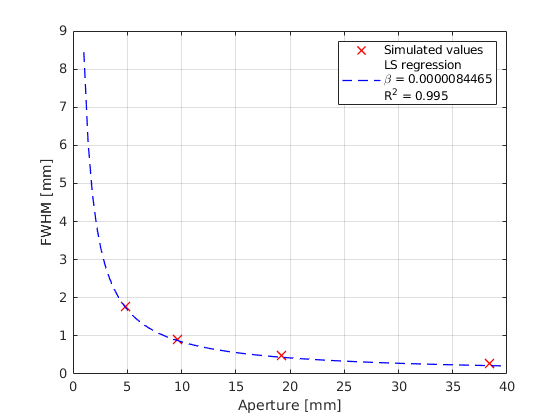
Plot the computed FWHM vs the active aperture width. Can you derive an empirical relation between the lateral FWHM of the PSF and L?
% The FWHM seems to be inversely proportional to the aperture size. We
% can confirm this hypotheis by doing a Least Squares (LS) regression using
% the model FWHM = beta/L. Values of R^2 close to 1 indicate that the
% model fits the data quite well.

beta=L/(1/FWHM.');
Lv=linspace(1e-3,40e-3,100);

R2 = 1 - sum((FWHM - beta./L).^2)/sum((FWHM - mean(FWHM)).^2);

figure('Color','w')
hold on
plot(L*1e3, FWHM*1e3, 'rx', 'LineWidth', 1, 'MarkerSize', 10)
plot(Lv*1e3, beta./Lv*1e3, 'b--', 'LineWidth', 1)
hold off
grid on
box on
xlabel('Aperture [mm]')
ylabel('FWHM [mm]')
legend('Simulated values', sprintf('LS regression\n\\beta = %.10f\nR^2 = %.3f', beta, R2))
Depth and lateral resolution
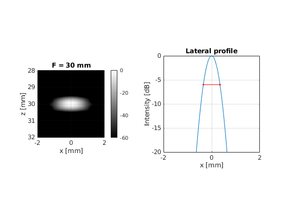
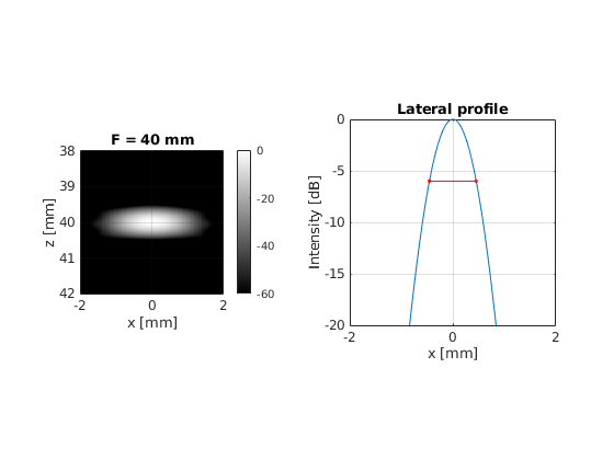
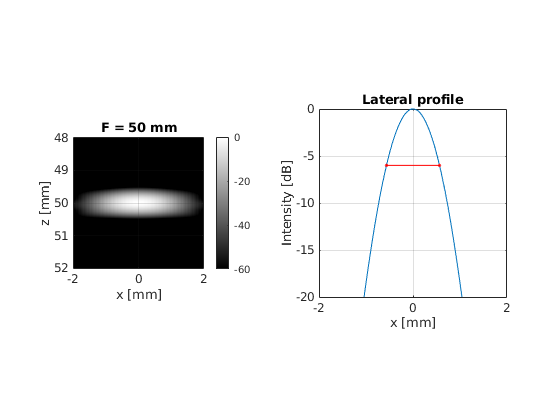
We also observed that the lateral resolution depends on the imaging depth. Let us study this quantitatively. We will calculate the FWHM along the lateral direction, but instead of changing the active aperture width we will change the distance of the point scatterer from the transducer. We will also change the focal depth accordingly.
Keeping a fixed 19.2 mm wide active aperture, set the focal depth to 10 mm, 20 mm, 30 mm, 40, and 50 mm. Beamform the images and calculate the lateral FWHM of the PSF.
% receive scan
N_scanlines=96;
x_axis=linspace(-2e-3, 2e-3, N_scanlines);

% probe
probe = uff.linear_array('N',128,...                % number elements
    'pitch',300e-6,...                              % pitch [m]
    'element_width',270e-6,...                      % element width [m]
    'element_height',4.5e-3);                       % element height [m]
% pulse
pulse = uff.pulse('center_frequency', 5.2e6,...     % center frequency [Hz]
    'fractional_bandwidth', 0.6);                   % fractional bandwidth [unitless]

% sequence
focal_depth = [20e-3, 30e-3, 40e-3, 50e-3];
L = 19.2e-3;                                        % Active aperture width
FWHM = zeros([1, length(focal_depth)]);

for i = 1:length(focal_depth)
    sequence = uff.wave();

    for n=1:N_scanlines
        % sequence definition
        sequence(n) = uff.wave();
        sequence(n).probe = probe;
        sequence(n).sound_speed=1540;

        % apodization
        xd=abs(probe.x-x_axis(n));                  % aperture distance [m]
        apodization = (double(xd<=L/2).*...
            (0.5 + 0.5*cos(2*pi*xd./L))).';      % apodization
        sequence(n).apodization = uff.apodization('apodization_vector',apodization);

        % source
        sequence(n).source=uff.point('xyz', [x_axis(n), 0, focal_depth(i)]);
    end

    % phantom
    Gamma=1;
    phantom = uff.phantom();
    phantom.points = [0,  0, focal_depth(i), Gamma];

    % simulation
    sim=fresnel();
    sim.phantom=phantom;            % phantom
    sim.pulse=pulse;                % transmitted pulse
    sim.probe=probe;                % probe
    sim.sequence=sequence;          % beam sequence
    sim.sampling_frequency=100e6;   % sampling frequency [Hz]
    channel_data=sim.go();

    % delay-and-sum (DAS) beamforming
    z_axis = channel_data.time*channel_data.sound_speed/2;
    delayed_data=zeros(size(channel_data.data));

    h = waitbar(0, 'Beamforming');
    for n=1:N_scanlines
        waitbar(n/N_scanlines, h);

        % we apply the same apodization function that we applied on transmit
        channel_data.data(:,:,n) = ...
            bsxfun(@times, channel_data.data(:,:,n), sequence(n).apodization.data.');

        for m=1:channel_data.N_channels
            % DRF
            distance=sqrt((probe.x(m)-x_axis(n)).^2+(probe.z(m)-z_axis(:)).^2)-z_axis(:);
            delay=distance./channel_data.sound_speed;

            % delay
            delayed_data(:,m,n)=interp1(channel_data.time, channel_data.data(:,m,n),...
                channel_data.time+delay,'linear',0);
        end
    end
    close(h)

    % sum
    b_image = squeeze(sum(delayed_data, 2));

    % envelope extraction
    envelope = abs(hilbert(b_image));

    % log compression
    envelope_dB = 20*log10(envelope/max(envelope(:)));

    figure('Color', 'w');
    subplot(1,2,1)
    imagesc(x_axis*1e3,z_axis*1e3,envelope_dB)
    axis equal tight
    ylim([-2, 2]+focal_depth(i)*1e3)
    xlim([-2, 2])
    colormap gray
    colorbar
    caxis([-60 0])
    xlabel('x [mm]')
    ylabel('z [mm]')
    title(sprintf('F = %.f mm', focal_depth(i)*1e3))
    box on
    grid on

    % get the profile
    [~, nz] = min(abs(z_axis-focal_depth(i)));
    profile = envelope_dB(nz,:);

    % we estimate location of the maximum
    [~, peak_index]=max(profile);

    % we obtain the -6dB point by interpolation
    x_6dB_l = interp1(profile(1:peak_index-1), x_axis(1:peak_index-1), -6, 'linear');
    x_6dB_r = interp1(profile(peak_index+1:end), x_axis(peak_index+1:end), -6, 'linear');

    % FWHM
    FWHM(i) = x_6dB_r - x_6dB_l;

    subplot(1,2,2);
    plot(x_axis*1e3,envelope_dB(nz,:))
    axis square tight
    ylim([-20, 0])
    xlim([-2, 2])
    grid on
    hold on
    box on
    plot([x_6dB_l, x_6dB_r]*1e3,[ -6 -6], 'r.-')
    xlabel('x [mm]')
    ylabel('Intensity [dB]')
    title('Lateral profile')
end

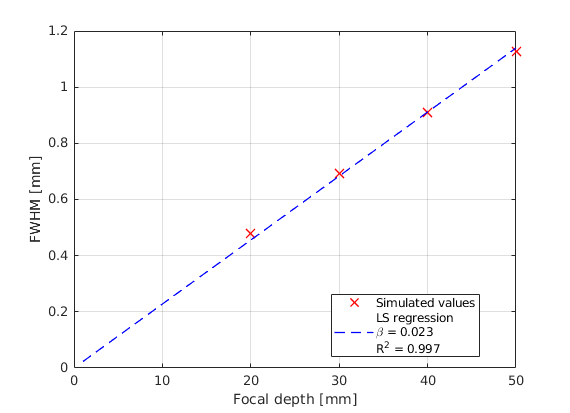
Plot the computed FWHM of the PSF vs the focal depth. What is the relation between them? Can you derive an empirical relation?
% The FWHM seems to be directly proportional to the depth. Once again, we
% can confirm this hypotheis by doing a Least Squares (LS) regression using
% the model FWHM = beta*F. Values of R^2 close to 1 indicate that the
% model fits the data quite well.

beta = FWHM/focal_depth;
R2 = 1 - sum((FWHM - beta.*focal_depth).^2)/sum((FWHM - mean(FWHM)).^2);

zv=linspace(1e-3,50e-3,100);

figure('Color','w')
hold on
plot(focal_depth*1e3,FWHM*1e3,'rx', 'LineWidth', 1, 'MarkerSize', 10)
plot(zv*1e3, zv*beta*1e3,'b--', 'LineWidth', 1)
hold off
grid on
box on
xlabel('Focal depth [mm]')
ylabel('FWHM [mm]')
legend('Simulated values', sprintf('LS regression\n\\beta = %.3f\nR^2 = %.3f', beta, R2), ...
    'location', 'best')
Expanding aperture
Now we know that lateral resolution is inversely proportional to the aperture size and directly proportional to the imaging depth. Let us define a new variable, called F-number (f#), as
For a fixed f#, the FWHM will be constant. Achieving homogenous image quality over the field of view is an important aspect in medical imaging. Using a fixed F-number for all depths allows us to control the lateral resolution and helps us fulfill this requirement.
Similarly to Dynamic Receive Focusing (DRF), expanding aperture can be implemented directly on receive without compromising the frame rate. It can also be implemented on transmit, if Multi Focus I+maging (MFI) is used. However, as we noted earlier, multi focus imaging leads to lower frame rate.
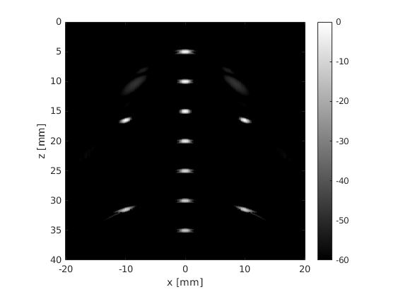
Let us implement expanding aperture on receive using 192 beams from -20 to 20 mm, using Hamming apodization both on transmit and receive. The focal depth is set to 15 mm. We will simulate a phantom consisting of several point scatterers, which resembles a commercial CIRS phantom.
Using an F-number f# = 1.5 on transmit and f# = 1.5 with expanding aperture on receive, beamform and plot the image
% phantom
phantom = uff.phantom();
phantom.points = [  0,      0, 5e-3, 1;
                    0,      0, 10e-3, 1;
                    0,      0, 15e-3, 1;
                    -10e-3, 0, 15e-3, 1;
                    10e-3,  0, 15e-3, 1;
                    0,      0, 20e-3, 1;
                    0,      0, 25e-3, 1;
                    0,      0, 30e-3, 1;
                    -10e-3, 0, 30e-3, 1;
                    10e-3,  0, 30e-3, 1;
                    0,      0, 35e-3, 1];

% sequence
N_scanlines=192;
x_axis=linspace(-20e-3, 20e-3, N_scanlines);
focal_depth = 15e-3;
sequence = uff.wave();
for n=1:N_scanlines
    % sequence definition
    sequence(n) = uff.wave();
    sequence(n).probe = probe;
    sequence(n).sound_speed=1540;

    sequence(n).apodization = uff.apodization('window', uff.window.hamming, ...
        'f_number', 1.5);
    sequence(n).source = uff.point('xyz', [x_axis(n), 0, 15e-3]);
    sequence(n).apodization.focus = uff.scan('xyz', [x_axis(n), 0, focal_depth]);
end

sim=fresnel();
sim.phantom=phantom;            % phantom
sim.pulse=pulse;                % transmitted pulse
sim.probe=probe;                % probe
sim.sequence=sequence;          % beam sequence
sim.sampling_frequency=100e6;   % sampling frequency [Hz]
channel_data=sim.go();

% delay-and-sum (DAS) beamforming
z_axis = channel_data.time*channel_data.sound_speed/2;
delayed_data = zeros(size(channel_data.data));
F_number_receive = 1.5;

h = waitbar(0, 'Beamforming');
for n=1:N_scanlines
    waitbar(n/N_scanlines, h);

    for m=1:channel_data.N_channels
        % DRF
        distance=sqrt((probe.x(m)-x_axis(n)).^2+(probe.z(m)-z_axis(:)).^2)-z_axis(:);
        delay=distance./channel_data.sound_speed;

        % Expanding aperture
        exp_aperture=z_axis/F_number_receive;
        xd=abs(probe.x(m)-x_axis(n));                         % aperture distance [m]
        receive_apodization=(double(xd<=exp_aperture/2).*...
            (0.5 + 0.5*cos(2*pi*xd./exp_aperture)));          % apodization

        % delay
        delayed_data(:,m,n)=interp1(channel_data.time, channel_data.data(:,m,n),...
            channel_data.time+delay,'linear',0) .* receive_apodization;
    end
end
close(h)

% sum
b_image = squeeze(sum(delayed_data, 2));

% envelope extraction
envelope = abs(hilbert(b_image));

% log compression
envelope_dB = 20*log10(envelope/max(envelope(:)));

figure('Color', 'w');
imagesc(x_axis*1e3, z_axis*1e3, envelope_dB)
axis equal tight
ylim([0, 40])
colormap gray
colorbar
caxis([-60 0])
xlabel('x [mm]')
ylabel('z [mm]')
box on