Transducer design¶

In this module we will study the basic concepts needed to design an ultrasound transducer with ceramic piezoelectric materials.

Related material:

Alfonso Rodriguez-Molares <alfonso.r.molares@ntnu.no>

Stefano Fiorentini <stefano.fiorentini@ntnu.no>

Last edit 3-10-2020

Slab thickness¶

We want to order a few Lead Zirconate Titanate (PZT) slabs to fabricate a single element transducer. We have chosen a PZT-8 material which has the following properties:

Young modulus: 7.1e10 N/m
Poisson’s ratio: 0.33
Density: 7700 kg/m3

Compute the speed of sound and the acoustic impedance of the material

Y = 7.1e10; 		% Young modulus [N/m]
nu = 0.33;  		% Poisson's ratio [unitless]
rho_PZT = 7700;     	% Density [kg/m3]

c_PZT = sqrt(Y*(1-nu)/rho_PZT/(1+nu)/(1-2*nu));
Z_PZT = rho_PZT*c_PZT*1e-6;

fprintf(1, ['Sound speed and acoustic impedance of PZT-8 are', ...
	'c_0 = %.2f m/s and Z = %.2f MRayl\n'], c_PZT, Z_PZT);

Sound speed and acoustic impedance of PZT-8 are c_0 = 3696.20 m/s and Z = 28.46 MRayl

Once the center frequency of the transducer \(f_0\) is chosen, the slab thickness that maximises the transducer sensitivity is given by

\[t_{PZT} = \frac{\lambda}{2} = \frac{c_0}{2 f_0}\]

In our example, the transducer will be used at a center frequency of 3 MHz.

What should be the thickness of the slab so that we get maximum output at the desired center frequency?

f0 = 3e6;            		% center frequency [Hz]

lambda = c_PZT/f0;   		% wavelength [m]
thickness = lambda/2; 		% thickness [m]

fprintf(1, 'The slab thickness should be %0.2f mm', thickness*1e3)

The slab thickness should be 0.61 mm

Harmonic analysis of a second order mechanical system¶

Before moving on to the next component in an ultrasound transducer, we will briefly introduce and analyse second-order mechanical systems. A second-order mechanical system consists of a mass \(m\), a spring with elastic coefficient \(k\), and a damper with damping coefficient \(b\). When the system is not under external excitation forces, it satisfies the differential equation

\[m\frac{d^2}{dt^2}x(t) + b\frac{d}{dt}x(t) + kx(t) = 0\]

This equation can be rearranged in the canonical form

\[\frac{d^2}{dt^2}x(t) + 2\xi w_0\frac{d}{dt}x(t) + w_0^2 x(t) = 0\]

where

\[w_0^2 = \frac{k}{m}\]

is the natural frequency of the mechanical system. In our case it is the center frequency of the transducer.

\[\xi = \frac{b}{2\sqrt{km}}\]

is the damping ratio of the mechanical system.

Since we are going to use this model to study the performance of an ultrasound transducer, it is more interesting to study the forced response of the system

\[\frac{d^2}{dt^2}x(t) + 2\xi w_0\frac{d}{dt}x(t) + w_0^2 x(t) = F(t)\]

where \(F(t)\) can be any kind of excitation function. However, due to the oscillatory nature of an ultrasound signal, we can focus our attention to periodic functions

\[F(t) = F_0 e^{jwt}\]

In other words, we are performing a harmonic analysis of the second-order mechanical system. To solve the second-order differential equation we assume that a solution exists in the form

\[x(t) = A e^{jwt} = |A| e^{j(wt + \phi)}\]

In words, we are assuming that the mass oscillates with the same frequency as the excitation function. Amplitude \(|A|\) and phase \(\phi\) of the oscillation depend instead on the properties of the second-order mechanical system. We substitute this definition for \(x(t)\) into the differential equation

\[-w_0^2 A e^{jwt} + j 2 \xi w_0 w A e^{jwt} + w_0^2 A e^{jwt} = \frac{F_0}{m} e^{jwt}\]

this equation can be solved for the unknown variable A

\[A = \frac{F_0 / m}{j 2 \xi w_0 w + (w_0^2 - w^2)}\]

This equation is often reffered to as a transfer function, because it describes how the output of the system (i.e. amplitude \(|A|\) and phase \(\phi\) of the oscillation) evolves when the input change. Assuming the natural frequency to be \(w_0\) = 3 MHz, plot the amplitude of the transfer function in dB in a range of frequencies between 0 MHz and 5 MHz, for damping ratios \(\xi\) = 0.1 and \(\xi\) = 0.5. You can normalise the plots by \(F_0 / k\), which is the value assumed by A at 0 Hz. Finally, calculate the -3dB bandwidth of the system.

f0 = 3e6;                                          % resonance frequency
xi = [0.1, 0.2];                                   % damping coefficient
    
f = 5e5:10:5e6;                                    % vector of evaluation frequencies

A = @(f, xi) 1 ./ (1j*2*xi*(2*pi*f0)*(2*pi*f) + ...
    ((2*pi*f0)^2 - (2*pi*f).^2));                  % transfer function

figure('Color', 'w')
hold on

for x = xi
    % Let us calculate the -3dB bandwidth of the transfer function
    
    f_3db_left = interp1(20*log10(abs(A(1e5:10:f0, x))/abs(A(f0, x))), 1e5:10:f0, -3);
    f_3db_right = interp1(20*log10(abs(A(f0:10:10e6, x))/abs(A(f0, x))), f0:10:10e6, -3);
    
    df = f_3db_right - f_3db_left;    
    
    plot(f, 20*log10(abs(A(f, x))/abs(A(0, x))), 'LineWidth', 1, 'DisplayName', ...
        sprintf('\\xi = %.1f', x))
    plot([f_3db_left; f_3db_right], [-3; -3]+20*log10(abs(A(f0, x))/abs(A(0, x))), ...
        'r-*', 'LineWidth', 1, 'DisplayName', sprintf('\\Deltaf = %.1f', df/f0))
end

hold off
set(gca, 'XScale', 'log', 'XTick', [1e6, f0], 'XTickLabel', {'1e6', 'f_0'})
grid on
box on
axis tight
xlabel('frequency [Hz]')
ylabel('abs(A) [dB]')
legend('location', 'northwest')

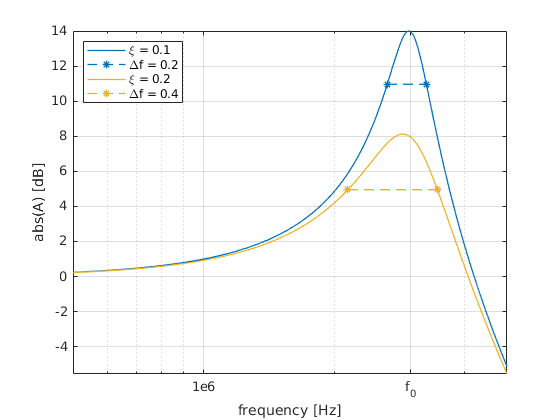
../../_images/second_order_system_analysis.png

the bandwidth of a second-order mechanical system (i.e. the ultrasound transducer we are trying to design) increases with the damping ratio \(\xi\). Moreover, the normalised bandwidth satisfies the relatio

\[\frac{\Delta f}{f_0} = 2 \xi\]

Q-factor. Backing layer¶

The Quality factor, or Q-factor, is an important property in the design of ultrasound transducers. The Q-factor can be defined as

\[Q = \frac{f_0}{\Delta f} = \frac{1}{2 \xi}\]

where \(f_0\) is the transducer center frequency and \(\Delta f\) is the transducer bandwidth. In our example, the manufacturer states that the material has a Q-factor of 800.

Calculate the bandwidth in Hz that we would obtain around the central frequency

Q=800;              % Mechanical Q-factor []
bandwidth=f0/Q;     % bandwidth [Hz]
disp(sprintf('The expected bandwidth is %0.2f kHz',bandwidth/1e3));

The expected bandwidth is 1.25 kHz

The pulse duration \(\Delta t\), expressed in seconds, can be approximated to

\[\Delta t \simeq \frac{1}{\Delta f}\]

Compute the axial resolution that we would obtain in water (c0 = 1500 m/s) if we used the material as it is

pulse_duration=1/bandwidth;  % pulse duration in [s]
c0=1500;                     % sound speed in water [m/s]
axial_resolution=c0*pulse_duration/2;
disp(sprintf('The expected axial resolution is %0.2f mm',axial_resolution*1e3));

The expected axial resolution is 600.00 mm

Unless we are designing a diagnostic system for dinosaurs, this kind of axial resolution is far from acceptable. In order to improve resolution we want to increase the transducer bandwidth, which means decreasing the Q-factor. By approximating the transducer to a second-order mechanical system, we predict that we can decrease the Q-factor by increasing the damping ratio \(\xi\). In practise this is achieved by adding a backing layer to the back side of the PZT. The backing layer absorbs the acoustic energy emitted by one side. Vibrations are attenuated faster, resulting in shorter pulses. The backing layer also provides a common support for the transducer elements. The acoustic impedance of the backing layer and the PZT should be similar to avoid reflections at the interface and maximise the effect of the backing layer. In our example, we would like the PZT + backing combination to achieve a 60% relative bandwith.

Compute the desired Q-factor of the PZT + backing combination

relative_bandwidth=0.6;             % relative bandwidth []
Q=1/relative_bandwidth;             % aimed Q-factor []
disp(sprintf('The Q-factor of the compound must be %0.2f',Q));

The Q-factor of the PZT + backing layer must be 1.67

Quarter-wavelength matching layer¶

The transducer will be used for medical applications. Human tissue has an acoustic impedance of \(Z_{T}\) = 1.54 MRayl.

Using the transmission coefficient, compute the relative amount of acoustic power that would be transferred from the transducer to the tissue

Z_tissue=1.54e6;        % Acoustic impedance of tissue [rayl/m2]
Z_PZT=rho_PZT*c_PZT;    % Acoustic impedance of PZT [rayl/m2]

Ri=((Z_tissue-Z_PZT)/(Z_tissue+Z_PZT)).^2;  % intensity reflection coefficient []
RTP=1-Ri;                                   % Relative transferred power []
disp(sprintf('Only %0.1f%% of the power is transferred ',RTP*100));

Only 19.5% of the total acoustic power is transferred

Almost 80% of the acoustic power is reflected back at the interface between the PZT transducer and the skin. This is not very efficient. However, we can improve the fraction of transmitted power by interposing an acoustic matching layer between transducer and tissue. As the name suggests, the role of the matching layer is to match two different acoustic impedances in order to maximise power transfer. It is possible to derive an analytical formula for the transmission coefficient between transducer and tissue when a matching layer is interposed.

\[T_I = \frac{4Z_{T}Z_{PZT}}{(Z_{PZT} + Z_{T})^2\cos^2(k t) + (Z_{ML} + \dfrac{Z_{PZT}Z_{T}}{Z_{ML}})^2\sin^2(k t)}\]

where \(k = 2\pi/\lambda\) is the wavenumber of the matching layer, \(t\) is the thickness of the matching layer, and \(Z_{PZT}\), \(Z_{ML}\), \(Z_{T}\) are the acoustic impedances of PZT, matching layer and tissue, respectively. In the next example we are going to see how the transmition coefficient changes with the thickness of the matching layer. We will assume the speed of sound in the matching layer to be \(c_{ML}\) = 3434 m/s and the acoustic impedance to be \(Z_{ML}\) = 10 MRayl.

Z_pzt = 28.46e6;            % Acoustic impedance of PZT [Rayl]
Z_t = 1.54e6;               % Acoustic impedance of tissue [Rayl]

Z_ml = 10e6;                % Acoustic impedance of matching layer [Rayl]
c_ml = 3434;                % Speed of sound of the matching layer [m/s]

f0 = 3e6;                   % Frequency value the matching layer is designed for [Hz]
lambda = c_ml/f0;           % Wavelength @ f0 in the matching layer
k = 2*pi/lambda;            % Wavenumber @ f0 in the matching layer

% Analytical expression for the transmission coefficient with a matching
% layer
T = @(t) 4*Z_pzt*Z_t ./ ((Z_pzt + Z_t)^2.*cos(k*t).^2 + ...
    (Z_ml + Z_pzt*Z_t./Z_ml).^2.*sin(k*t).^2);

% Plot
t = linspace(0, lambda, 1e3);

figure('Color', 'w')
plot(t/lambda, T(t), 'LineWidth', 1)
axis tight
grid on
box on
xlabel('thickess / \lambda [adim]')
ylabel('transmission coefficient [adim]')

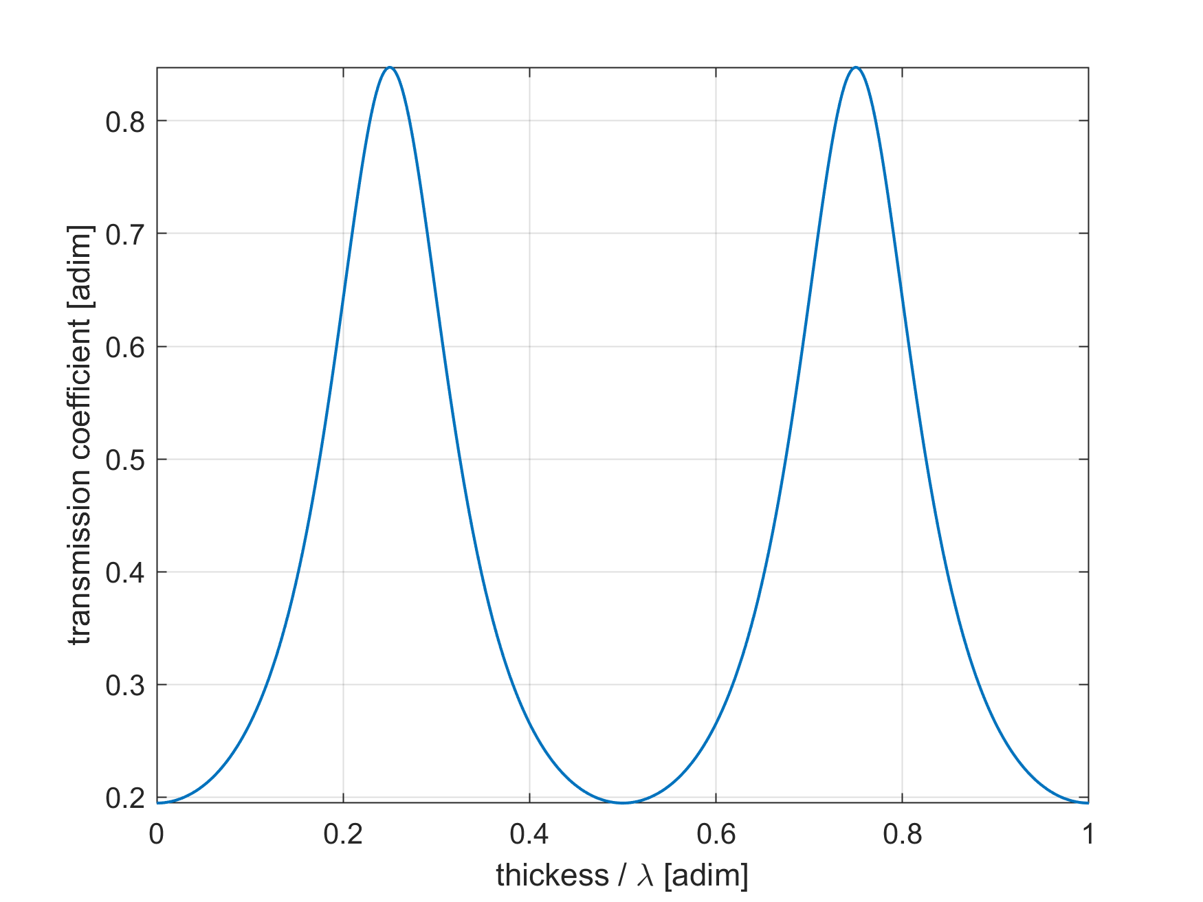
../../_images/matching_layer_thickness.png

We can see that the transmission coefficient reaches a maximum when the thickness of the matching layer satisfies the relation

\[t_{ML} = (2n + 1)\frac{\lambda}{4}, n \in \mathbb{N}\]

Remember that the wavelength \(\lambda\) must be calculated using the speed of sound of the matching layer. The most common choice for the thickness is \(\lambda/4\), hence its name. At high frequencies it may be too difficult to manifacture a matching layer with a thickness of \(\lambda/4\). In these cases, a thickness of \(t_{ML} = 3\lambda/4\) can also be used, although with reduced performance. In the previous example we have seen that a value of the acoustic impedance of 10 MRayl achieved a transmission coefficient around 80%. Not bad, but can we do any better?

Z_pzt = 28.46e6;            % Acoustic impedance of PZT [Rayl]
Z_t = 1.54e6;               % Acoustic impedance of tissue [Rayl]

c_ml = 3434;                % Speed of sound of the matching layer [m/s]

f0 = 3e6;                   % Frequency value the matching layer is designed for [Hz]
lambda = c_ml/f0;           % Wavelength @ f0 in the matching layer
k = 2*pi/lambda;            % Wavenumber @ f0 in the matching layer

t = lambda / 4;             % Thickness of the matching layer [m]

% Analytical expression for the transmission coefficient with a matching
% layer
T = @(Z_ml) 4*Z_pzt*Z_t ./ ((Z_pzt + Z_t)^2.*cos(k*t).^2 + ...
    (Z_ml + Z_pzt*Z_t./Z_ml).^2.*sin(k*t).^2);

% Plot
Z_ml = linspace(Z_t, Z_pzt, 1e3);    % Acoustic impedance of matching layer [Rayl]

figure('Color', 'w')
plot(Z_ml*1e-6, T(Z_ml), 'LineWidth', 1)
axis tight
grid on
box on
xlabel('Z_{ML} [MRayl]')
ylabel('transmission coefficient [adim]')

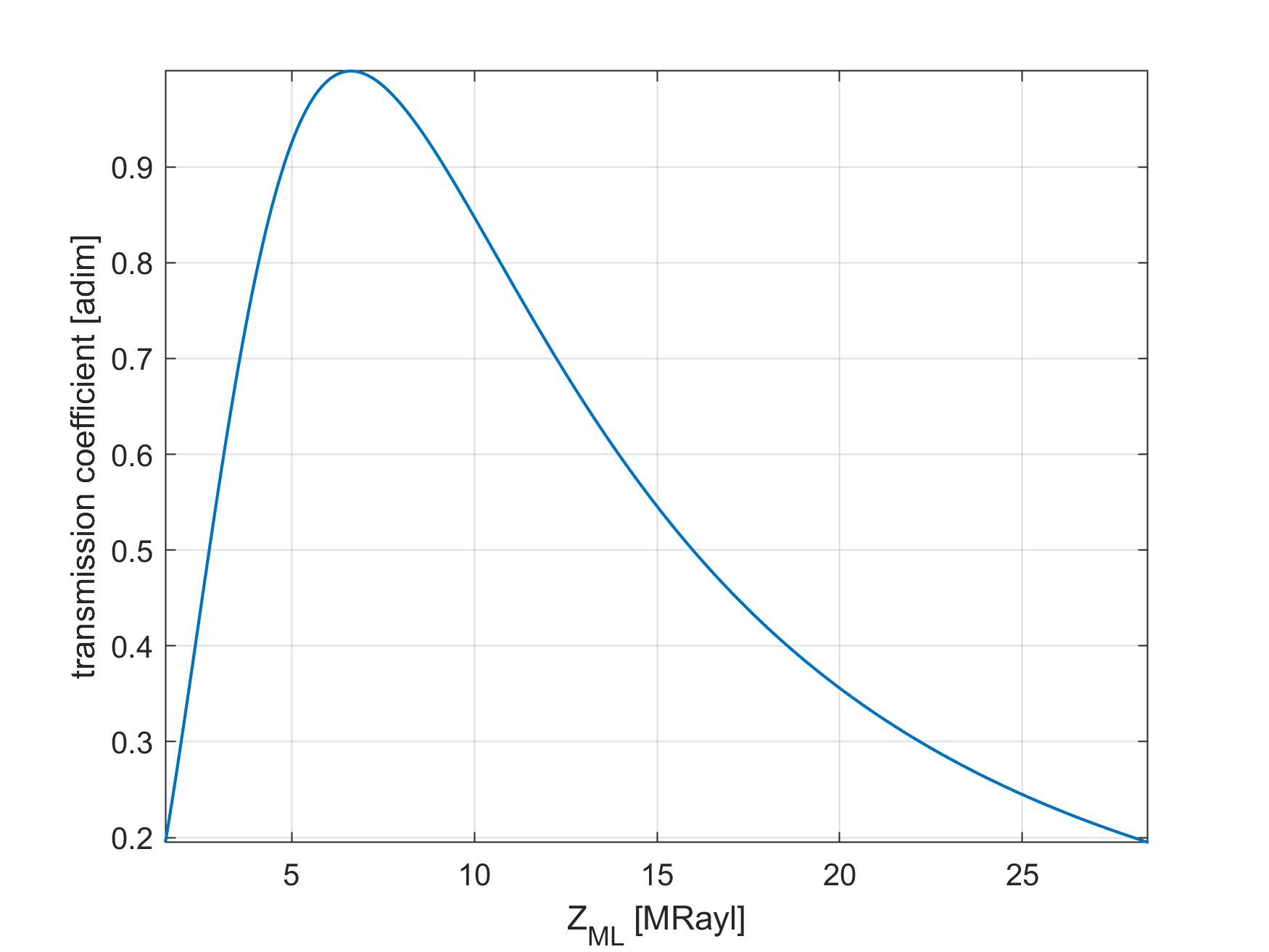
The previous examples shows that, for an acoustic impedance of the matching layer equal to

\[Z_{ML} = \sqrt(Z_{PZT}Z_{tissue})\]

the transmit coefficient becomes 1, meaning that all of the acoustic power is transferred from the transducer to the tissue. As a final note, lets see how the matching layer that we have just designed behaves in a range of frequencies.

Z_pzt = 28.46e6;            % Acoustic impedance of PZT [Rayl]
Z_t = 1.54e6;               % Acoustic impedance of tissue [Rayl]

Z_ml = sqrt(Z_pzt*Z_t);    % Acoustic impedance of the matching layer [Rayl]
c_ml = 3434;                % Speed of sound of the matching layer [m/s]

f0 = 3e6;                   % Frequency value the matching layer is designed for [Hz]
lambda = c_ml/f0;           % Wavelength @ f0 in the matching layer
t = lambda / 4;             % Thickness of the matching layer [m]

% Analytical expression for the transmission coefficient with a matching
% layer
k = @(f) 2*pi*f/c_ml;       % Wavenumber @ f

T = @(f) 4*Z_pzt*Z_t ./ ((Z_pzt + Z_t)^2.*cos(k(f)*t).^2 + ...
    (Z_ml + Z_pzt*Z_t./Z_ml).^2.*sin(k(f)*t).^2);

% Plot
f = linspace(f0/2, 3*f0/2, 1e3);

figure('Color', 'w')
plot(f*1e-6, T(f), 'LineWidth', 1)
axis tight
grid on
box on
xlabel('f [MHz]')
ylabel('transmission coefficient [adim]')

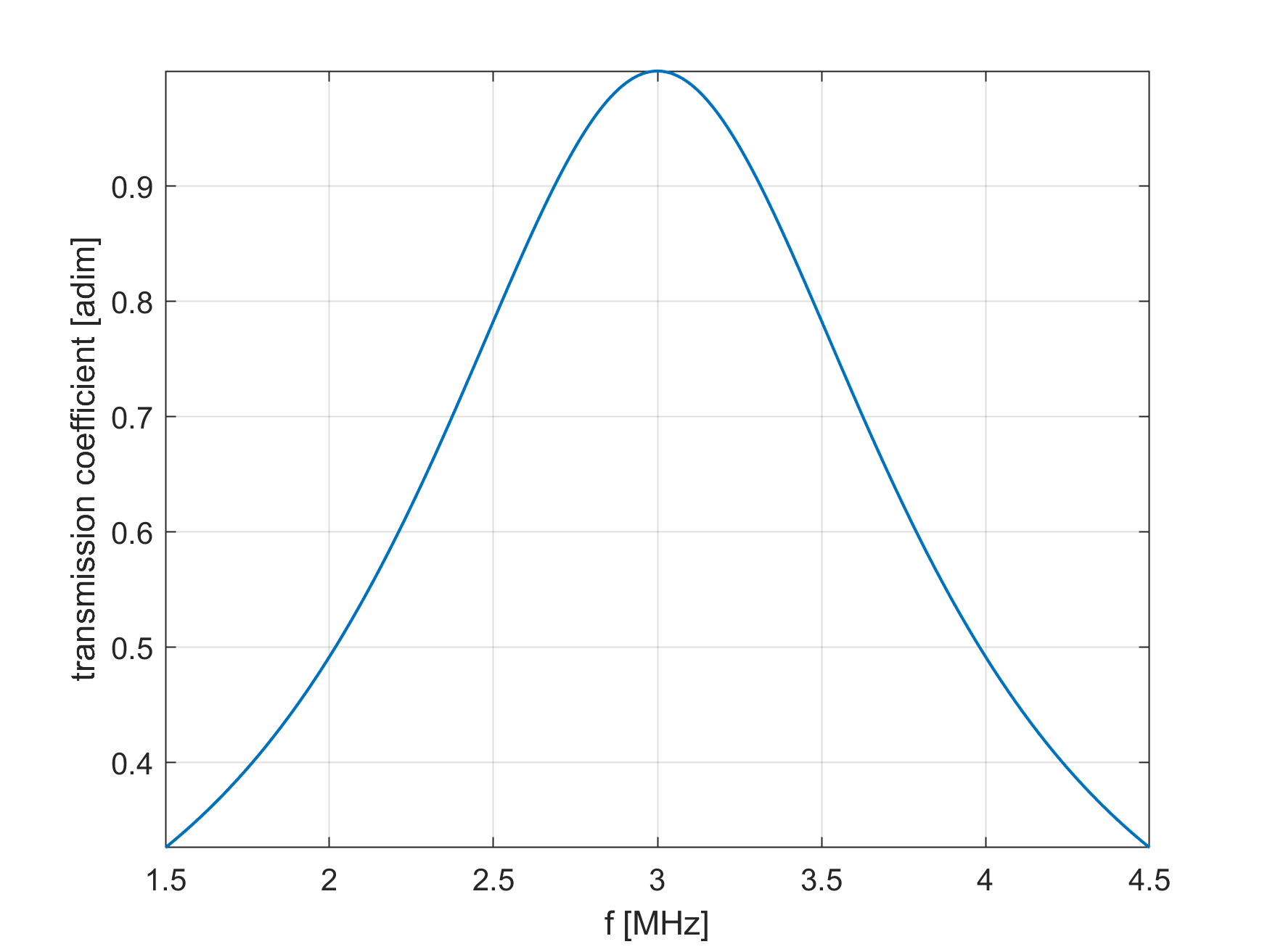
Unfortunately the matching layer works best for a small range of frequencies that satisfy

\[f \simeq \frac{c_{ML}}{t_{ML}}\]

In other words, the matching layer acts as a mechanical bandpass filter which reduces the bandwidth of the backing layer + PZT combination. To mitigate this issue, two or more matching layers with different thicknesses (and therefore frequency ranges) and acoustic impedances may be used in high end medical transducers. How thickess and acoustic impedance are designed for such configurations is beyond the scope of this course.

Excercise: We excite the transducer above with an ideal sinc pulse with a base frequency of 3 MHz and a bandwidth of 1 MHz. Sketch the frequency spectrum of the transmitted acoustic pulse. How will this affect the transmitted signal in the time domain?