Safety
We analyze data acquired with the hydrophone scanning system. The data was recorded to study the safety of probe L11-4v and the Verasonic platform using a plane wave sequence.
Related materials:
by Alfonso Rodriguez-Molares (alfonso.r.molares@ntnu.no) 06.11.2016
Contents
- Axis scan
- Acoustic working frequency
- Time averaged intensity integral
- Derated time averaged intensity integral
- Derated peak rarefactional pressure
- Mechanical index
- Output beam area and breakpoint distance
- Raster scan
- Acoustic power
- Attenuated acoustic power
- Depth for TIS
- TIS, below surface, non-scanning
- Depth for TIB
- TIB, below surface, non-scaning
- TIC, non-scaning
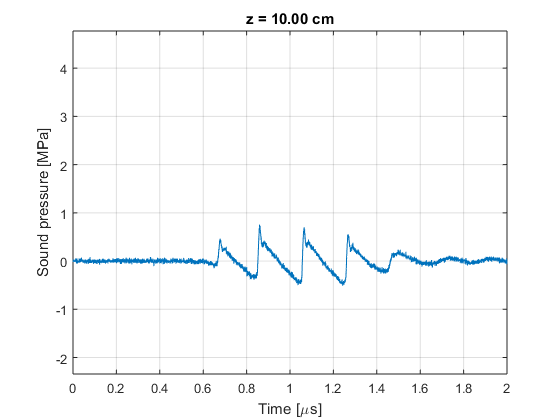
Axis scan
We recorded an axis scan, storing all the pulses (or waveforms) at different distances from the probe. You can download the data here:
- Load the data and make a video of the waveform at different depths
% we load the data
load('axis_scan.mat');

% some variables
z_axis=xyz(3,:);    % z-axis [m]

% we loop over the depth vector
figure;
for n=1:numel(z_axis)
    plot(t*1e6,p(:,n)/1e6); grid on; hold off;
    ylim([min(p(:)/1e6) max(p(:)/1e6)]);
    xlabel('Time [\mus]');
    ylabel('Sound pressure [MPa]');
    title(sprintf('z = %0.2f cm',z_axis(n)*1e2));
    pause(0.1);
end
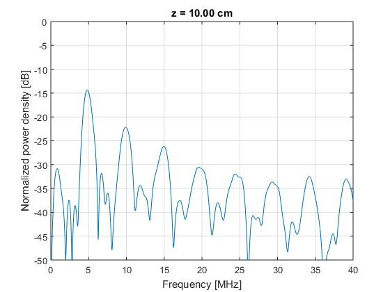
- Compute the FFT and make a video of the power spectrum at different depths
% compute FFT
Ts=t(2)-t(1);                   % Sampling interval [s]
Fs=1/Ts;                        % Sampling frequency [Hz]

NFFT=1e6;                       % we increase the number of samples for visualization purposes
p_fft=fft(p,NFFT);              % compute the fft
P_fft=abs(p_fft).^2;            % power density [dB]
P_fft_dB=10*log10(P_fft./max(P_fft(:)));  % power density [dB]
f_vector=(0:NFFT-1)/NFFT*Fs;    % frequency vector [Hz]

% we loop over the depth vector
figure;
for n=1:numel(z_axis)
    plot(f_vector/1e6,P_fft_dB(:,n)); grid on; hold off;
    ylim([-50 0]);
    xlabel('Frequency [MHz]');
    ylabel('Normalized power density [dB]');
    xlim([0 40]);
    title(sprintf('z = %0.2f cm',z_axis(n)*1e2));
    pause(0.1);
end
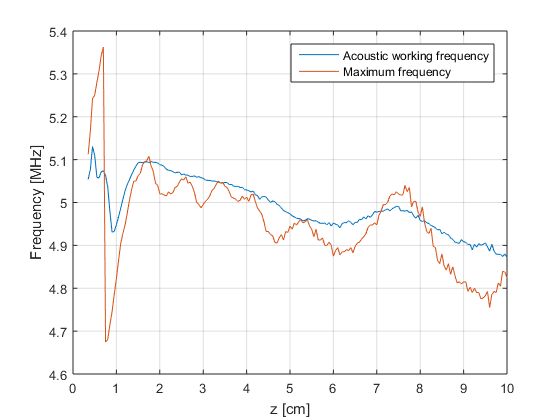
Acoustic working frequency
- Estimate the acoustic working frequency at different depths
% crop values
mask=f_vector<40e6;                     % we only keep the samples in a reasonable range
p_fft=p_fft(mask,:);
f_vector=f_vector(mask);

% we loop over the depth vector
figure;
for n=1:numel(z_axis)
    [pmax ind]=max(abs(p_fft(:,n)));
    f_max(n)=f_vector(ind);
    p_dB=20*log10(abs(p_fft(:,n))./pmax);
    mask_up=(f_vector>f_max(n))&(p_dB>-12).';
    f_bw_up=interp1(p_dB(mask_up),f_vector(mask_up),-6);
    mask_down=(f_vector<f_max(n))&(p_dB>-12).';
    f_bw_down=interp1(p_dB(mask_down),f_vector(mask_down),-6);
    f_awf(n)=(f_bw_up+f_bw_down)/2;

%     plot(f_vector/1e6,p_dB); grid on; hold on;
%     plot(f_max(n)/1e6,0,'ro');
%     plot(f_awf(n)/1e6,0,'b+');
%     ylim([-50 0]);
%     xlabel('Frequency [MHz]');
%     ylabel('Normalized power density [dB]');
%     xlim([0 40]);
%     title(sprintf('z = %0.2f cm',z_axis(n)*1e2));
%     pause(0.1); hold off;
end

figure;
plot(z_axis*1e2,f_awf/1e6); grid on; hold on;
plot(z_axis*1e2,f_max/1e6);
legend('Acoustic working frequency','Maximum frequency');
xlabel('z [cm]');
ylabel('Frequency [MHz]');

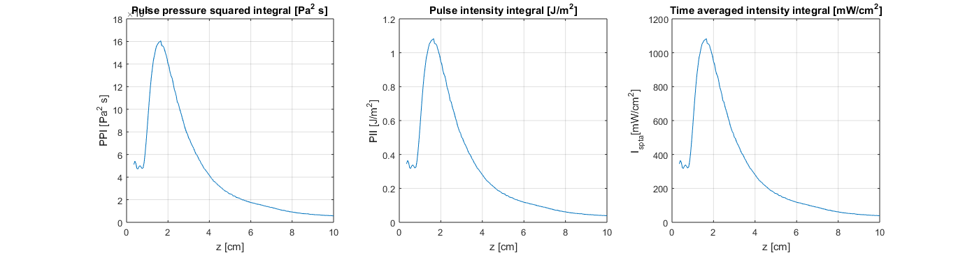
Time averaged intensity integral
At the measured temperature the water density is 998 kg/m3 and the speed of sound is 1485.2 m/s. The probe uses a quite high pulse repetition frequency (PRF): 10 kHz.
- Compute and plot: # pulse pressure squared integral [Pa2 s], # pulse intensity integral [J/m2], and # time averaged intensity integral [mW/cm2].
% input quantities
rho=998.0;                              % density [kg/m3]
c=1485.2;                               % speed of sound [m/s]
PRF=10e3;                               % pulse repetition frequency [Hz]

PPI=sum(p.^2,1)*Ts;                     % Pulse pressure squared integral [Pa^2*s]
PII=PPI/rho/c;                          % Pulse intensity integral [J/m^2]
Ispta=PII.*PRF;                         % Time averaged intensity integral [W/m^2]

figure;
subplot(1,3,1);
plot(z_axis*1e2,PPI); hold on; grid on;
xlabel('z [cm]');
ylabel('PPI [Pa^2 s]');
title('Pulse pressure squared integral [Pa^2 s]');

subplot(1,3,2);
plot(z_axis*1e2,PII); hold on; grid on;
xlabel('z [cm]');
ylabel('PII [J/m^2]');
title('Pulse intensity integral [J/m^2]');

subplot(1,3,3);
plot(z_axis*1e2,Ispta/10); hold on; grid on;
xlabel('z [cm]');
ylabel('I_{spta}[mW/cm^2]');
title('Time averaged intensity integral [mW/cm^2]');
set(gcf,'Position',[258 244 1390 363])
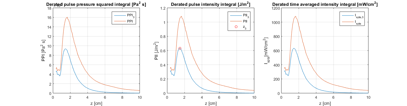
Derated time averaged intensity integral
Assume a attenuation coefficient of 0.3 dB/cm/MHz.
- Compute and plot: # derated pulse pressure squared integral [Pa2 s], # derated pulse intensity integral [J/m2], and # derated time averaged intensity integral [mW/cm2].
% attenuation
alpha=0.3;                                            % attenuation coefficient [dB/cm/MHz]
att_power=10.^-(alpha*(z_axis/1e-2).*(f_awf/1e6)/10);   % attenuation factor

% derated quantities
PPI_3=PPI.*att_power;                                 % attenuated pulse pressure squared integral [Pa^2*s]
PII_3=PII.*att_power;                                 % attenuated pulse intensity integral [J/m^2]
Ispta_3=Ispta.*att_power;                             % attenuated Time averaged intensity integral [W/m^2]

figure;
subplot(1,3,1);
plot(z_axis*1e2,PPI_3); hold on; grid on;
plot(z_axis*1e2,PPI);
xlabel('z [cm]');
ylabel('PPI [Pa^2 s]');
title('Derated pulse pressure squared integral [Pa^2 s]');
legend('PPI_{3}','PPI');

subplot(1,3,2);
plot(z_axis*1e2,PII_3); hold on; grid on;
plot(z_axis*1e2,PII);
plot(z3*1e2,PII_3_max,'ro')
xlabel('z [cm]');
ylabel('PII [J/m^2]');
title('Derated pulse intensity integral [J/m^2]');
legend('PII_{3}','PII','z_3');

subplot(1,3,3);
plot(z_axis*1e2,Ispta_3/10); hold on; grid on;
plot(z_axis*1e2,Ispta/10);
xlabel('z [cm]');
ylabel('I_{spta}[mW/cm^2]');
title('Derated time averaged intensity integral [mW/cm^2]');
legend('I_{spta,3}','I_{spta}');
set(gcf,'Position',[258 244 1390 363])
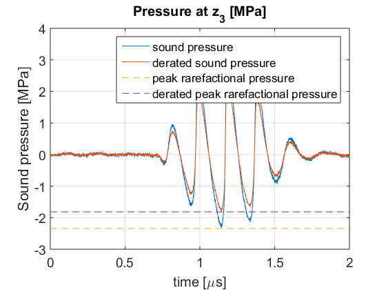
Derated peak rarefactional pressure
- Compute the depth
 of the maximum derated time averaged intensity integral
% calculation z3
[PII_3_max z3_index]=max(PII_3);
z3=z_axis(z3_index);
disp(sprintf('z3: %0.2f cm',z3*100));
z3: 1.45 cm
- Compute the derated peak rarefactional pressure [MPa] at said
% to derate pressure we need a different attenuation expression
att_press=10.^-(alpha*(z3/1e-2).*(f_awf(z3_index)/1e6)/20);         % attenuation factor -> BEWARE OF THE 2 FACTOR ON THE DENOMINATOR

% peak rarefactional pressure
p_z3=p(:,z3_index);                            % sound pressure at z3 [Pa]
pr=max(-p_z3);                                 % peak rarefactional pressure (Pa)
pr3=max(-p_z3.*att_press);                       % derated peak rarefactional pressure (Pa)

figure;
plot(t*1e6,p_z3./1e6); hold on; grid on;
plot(t*1e6,p_z3.*att_press./1e6);
plot([0 max(t)*1e6],-[pr pr]./1e6,'--');
plot([0 max(t)*1e6],-[pr3 pr3]./1e6,'--');
xlabel('time [\mus]');
ylabel('Sound pressure [MPa]');
legend('sound pressure','derated sound pressure','peak rarefactional pressure','derated peak rarefactional pressure');
title(sprintf('Pressure at z_3 [MPa]'));
set(gca,'FontSize',14);
Mechanical index
- Compute the Mechanical Index
if(f_awf(z3_index)<4e6)
    MI=(pr3/1e6)/sqrt((f_awf(z3_index)/1e6));       % Mechanical index (unitless) for fawf<4MHz
else
    MI=(pr3/1e6)/2;                                 % Mechanical index (unitless) for fawf>4MHz
end
disp(sprintf('MI: %0.1f',MI));
MI: 0.9
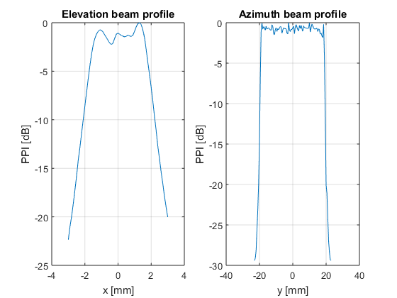
Output beam area and breakpoint distance
To study the probe aperture two linear scans were recorded crossing the center of the aperture through the x and y axis at a 4 mm depth. You can download the data here:
The data contains the pulse pressure integral (PPI) in dB. And just to make the things more interesting the x-axis, which we normally assign to the azimuth, is actually elevation. And the y-axis is assigned to azimuth.
- * Load the data and represent the beam profiles*
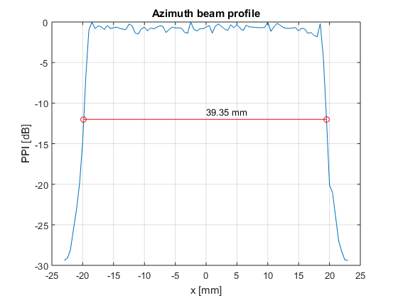
% load the data
load('beam_profile.mat');

% show
figure;
subplot(1,2,1)
plot(el_xyz(1,:)*1e3,el_profile); grid on; hold on;
xlabel('x [mm]');
ylabel('PPI [dB]');
title('Elevation beam profile');

subplot(1,2,2)
plot(az_xyz(2,:)*1e3,az_profile); grid on; hold on;
xlabel('y [mm]');
ylabel('PPI [dB]');
title('Azimuth beam profile');
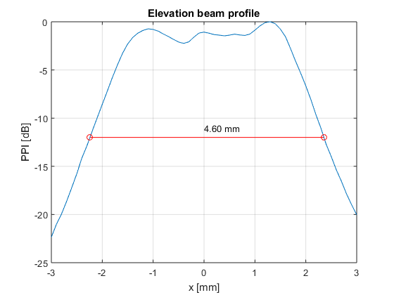
- Compute the -12 dB ouput beam area
% compute the -12 dB aperture height
n_over_12=find(el_profile>=-12);        % get the positions with intensity greater than -12 dB
n_up=max(n_over_12);                    % location of the upper limit
x_up=interp1([el_profile(n_up) el_profile(n_up+1)],[el_xyz(1,n_up) el_xyz(1,n_up+1)],-12); % linear interpolation for greater precision
n_down=min(n_over_12);                  % location of the lower limit
x_down=interp1([el_profile(n_down-1) el_profile(n_down)],[el_xyz(1,n_down-1) el_xyz(1,n_down)],-12); % linear interpolation for greater precision
Height=x_up-x_down;                         % -12dB aperture height [m]

figure;
plot(el_xyz(1,:)*1e3,el_profile); grid on; hold on;
plot([x_down x_up]*1e3,[-12 -12],'ro-');
text(0,-11,sprintf('%0.2f mm',Height*1e3));
xlabel('x [mm]');
ylabel('PPI [dB]');
title('Elevation beam profile');

% compute the -12dB aperture width
n_over_12=find(az_profile>=-12);        % get the positions with intensity greater than -12 dB
n_up=max(n_over_12);                    % location of the upper limit
y_up=interp1([az_profile(n_up) az_profile(n_up+1)],[az_xyz(2,n_up) az_xyz(2,n_up+1)],-12); % linear interpolation for greater precision
n_down=min(n_over_12);                  % location of the lower limit
y_down=interp1([az_profile(n_down-1) az_profile(n_down)],[az_xyz(2,n_down-1) az_xyz(2,n_down)],-12); % linear interpolation for greater precision
Width=y_up-y_down;                         % -12dB aperture width [m]

figure;
plot(az_xyz(2,:)*1e3,az_profile); grid on; hold on;
plot([y_down y_up]*1e3,[-12 -12],'ro-');
text(0,-11,sprintf('%0.2f mm',Width*1e3));
xlabel('x [mm]');
ylabel('PPI [dB]');
title('Azimuth beam profile');

% -12 dB output beam area
Aaprt=Height*Width;  % -12dB output beam area [m^2]
disp(sprintf('-12 dB output beam area = %0.2f cm^2',Aaprt*1e4))
-12 dB output beam area = 1.81 cm^2
- Compute the breakpoint distance
% breakpoint distance
Deq=max(sqrt(4/pi*Aaprt),1e-3);         % Equivalent aperture diameter [m]
z_bp=1.5*Deq;                           % breakpoint distance [m]
disp(sprintf('Breakpoint distance = %0.2f cm',z_bp*1e2))
Breakpoint distance = 2.28 cm
Raster scan
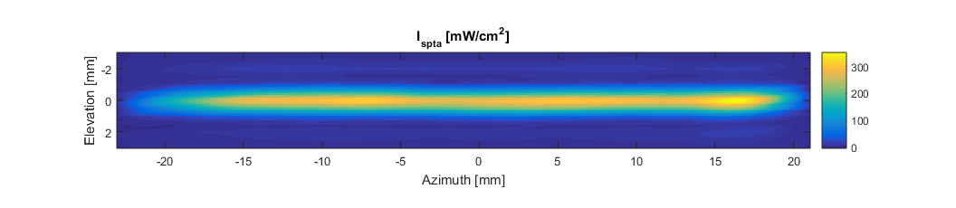
A raster scan, a scan across the beam area, was performed at a distance greater than the breakpoint distance. The data can be downloaded from:
The data contains the sound pressure in [Pa].
- Load the data and show a map of the

% load data
load('raster_scan.mat');

% compute the intensity
I=sum(p.^2,1)*Ts/rho/c*PRF;                % Time-averaged acoustic intensity (W/m^2)

% spatial interpolation of the intensity (not necesary but cool)
dr=0.1e-3;                                      % regular interpolation distance (m)
x=min(xyz(1,:)):dr:max(xyz(1,:));               % x-vector (m)
y=min(xyz(2,:)):dr:max(xyz(2,:));               % y-vector (m)
[Xi Yi]=meshgrid(x,y);                          % 2D vectors (m)
Ii=griddata(xyz(1,:),xyz(2,:),I,Xi,Yi,'cubic'); % interpolated intensity (W/m^2)
assert(~sum(isnan(Ii(:))),'The interpolated time averaged acoustic intensity has holes! Check the interpolation please.');

figure;
imagesc(y*1e3,x*1e3,Ii.'/10); axis equal tight;
xlabel('Azimuth [mm]');
ylabel('Elevation [mm]');
colorbar;
title('I_{spta} [mW/cm^2]');
set(gcf,'Position',[488         532        1056         230]);
Acoustic power
By integrating the time averaged intensity integral () over the raster area the acoustic power  emitted by the transducer can be estimated.
- Estimate the acoustic power
P=sum(Ii(:)).*dr.^2;                             % Acoustic power (W)
disp(sprintf('Acoustic power: %0.2f mW',P*1e3));
Acoustic power: 152.51 mW
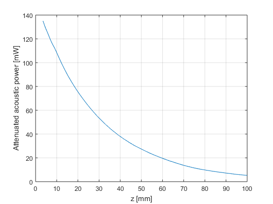
Attenuated acoustic power
I tissue with a attenuation coefficient of 0.3 dB/cm/MHz the acoustic power will decrease with depth.
- Estimate and plot the attenuated acoustic power with depth
P3=P.*att_power;                                       % derated power (W)

figure;
plot(z_axis*1e3,P3*1e3); grid on;
xlabel('z [mm]');
ylabel('Attenuated acoustic power [mW]');
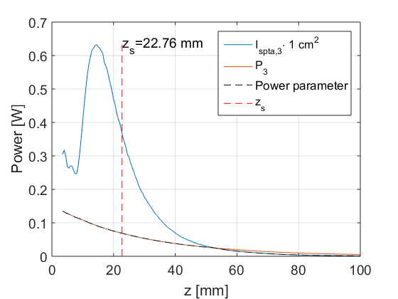
Depth for TIS
The standard IEC 62359 states that the soft tissue thermal index model must be calculated at a certain depth denoted as  . This depth is described in the standard IEC 62359 as:
"the distance along the beam axis from the external transducer aperture to the plane at which the lower value of the attenuated output power and the product of the attenuated spatial-peak temporal-average intensity and 1 cm2 is maximized over the distance range equal to, or greater than, the break-point depth"
- Decipher that and compute
% Calculate z_s
zs_function=min([P3;Ispta_3*(1e-2)^2]);         % power parameter to claculate zs (W)
[mm ii]=max(zs_function);                       % maximum of the power parameter (W)
zs=max(z_axis(ii),z_bp);                        % zs (m)

figure;
plot(z_axis*1e3,Ispta_3*(1e-2)^2); hold on; grid on;
plot(z_axis*1e3,P3);
plot(z_axis*1e3,zs_function,'k--');
plot([zs zs]*1e3,[0 max(Ispta_3*1e-4)],'r--');
text(zs*1e3,max(Ispta_3*(1e-2)^2),sprintf('z_s=%0.2f mm',zs*1e3),'FontSize',14);
xlabel('z [mm]');
ylabel('Power [W]');
legend('I_{spta,3}\cdot 1 cm^2','P_3','Power parameter','z_s');
set(gca,'FontSize',14)
TIS, below surface, non-scanning
The sequence is non-scaning. The soft tissue thermal index below the surface is computed as:
![$TIS= \min \left( \frac{P_3(z_s) f_{awf}}{2.1e5 [W Hz]}, \frac{I_{spta,3}(z_s) f_{awf}}{2.1e9 [W Hz/m^2]} \right)$](exercise_safety_eq01135942393667995733.png)
- Compute the TIS below the surface
P3_zs=interp1(z_axis,P3,zs);
Ispta_3_zs=interp1(z_axis,Ispta_3,zs);
f_awf_zs=interp1(z_axis,f_awf,zs);
TIS=min([P3_zs*f_awf_zs/2.1e5],[Ispta_3_zs*f_awf_zs/2.1e9]);
disp(sprintf('TIS: %0.1f',TIS));
TIS: 1.7
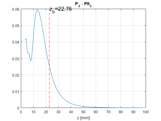
Depth for TIB
The standard IEC 62359 states that the bone at focus thermal index model must be calculated at a certain depth denoted as  . This depth is described in the standard IEC 62359 as:

- Compute
% calculate zb
zb_function=P3.*PII_3;
[mm ii]=max(zb_function);
zb=max([ z_bp z_axis(ii)]);

figure;
plot(z_axis*1e3,zb_function); hold on; grid on;
plot([zb zb]*1e3,[0 mm],'r--');
text(zb*1e3,mm,sprintf('z_b=%0.2f',zb*1e3),'FontSize',14);
xlabel('z [mm]');
title('P_3 \cdot PII_3');
TIB, below surface, non-scaning
The bone at focus thermal index below the surface is computed as:
![$TIB= \textmd{min} \left( \frac{ \sqrt{ P_3(z_b) I_{spta,3}(z_b)} }{5 [W/m]}, \frac{P_{3}(z_b)}{4.4e^{-3} [W]} \right)$](exercise_safety_eq05608578921364925653.png)
- Compute the TIB below the surface
P3_zb=interp1(z_axis,P3,zb);
Ispta_3_zb=interp1(z_axis,Ispta_3,zb);
TIB=min([sqrt(P3_zb*Ispta_3_zb)/5, P3_zb/4.4e-3]);
disp(sprintf('TIB: %0.1f',TIB));
TIB: 3.2
TIC, non-scaning
Logically, the bone thermal index at surface equals the cranial thermal index . For non-scaning modes the TIC is calculated as:
![$TIC=\frac{P}{D_{eq} 4 [W/m]}$](exercise_safety_eq02280276588069497181.png)
- Compute the TIC
TIC=P/Deq/4;
disp(sprintf('TIC: %0.1f',TIC));

disp('------------');
disp(sprintf('MI : %0.1f',MI));
disp(sprintf('TIS: %0.1f',TIS));
disp(sprintf('TIB: %0.1f',TIB));
disp(sprintf('TIC: %0.1f',TIC));
disp('------------');
TIC: 2.5
------------
MI : 0.9
TIS: 1.7
TIB: 3.2
TIC: 2.5
------------