Physics - Pitch-Catch
This exercise is just a small variation on the previous one, but serves us to introduce the first deliverable of the course. Don't blink
Related materials:
by Alfonso Rodriguez-Molares (alfonso.r.molares@ntnu.no) 21.07.2016
Contents
Two transducers
Based on the model we introduced in the previous exercise now we would like to examine the impulse response of a system with two transducers in a pitch-catch configuration, this is, one acting only as transmitter and the other acting only as receiver. Let us denote  the position where the transmitting element is and
  the position where the receiving element is. Let us assume there is a point reflector at point
  with a reflection coefficient
  .
.
- Derive the two-way impulse response
% Easy peasy.
%
% $h(t,\mathbf{s},\mathbf{r}) = \Gamma \frac{\delta(t-(r_T+r_R)/c_0)}{4\pi r_T r_R} \, D(\theta_T,\phi_T) D(\theta_R,\phi_R)$
%
% where
%
% $r_T=||\mathbf{t}$ - $\mathbf{p}||$,
% $r_R=||\mathbf{p}$ - $\mathbf{r}||$,
% $\theta_T=\arctan\left(\frac{P(1)-T(1)}{P(3)-T(3)}\right)$
% $\phi_T=  \arctan\left(\frac{P(2)-T(2)}{P(3)-T(3)}\right)$
% $\theta_R=\arctan\left(\frac{P(1)-R(1)}{P(3)-R(3)}\right)$
% $\phi_R=  \arctan\left(\frac{P(2)-R(2)}{P(3)-R(3)}\right)$
Using a Gaussian-modulated RF signal
 .
.
where  = 4 MHz,
  , and
, and  =80 MHz. Consider two identical transducers
  =1 mm wide,
  =5 mm tall. One transducer is at the origin of coordinates with its face pointing downwards (towards positive z). The other is placed at (10,0,0) mm also pointed downwards. A point scatterer exists at
  =(0,0,20) with reflection coefficient
  =1.
=1.
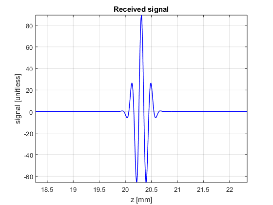
- Simulate the received signal and plot it (the signal not the amplitude)
f=4e6;                              % transducer frequency [MHz]
Deltaf=0.6*f;                       % pulse bandwidth [MHz]
c0=1540;                            % speed of sound [m/s]
lambda=c0/f;                        % wavelength [m]
k=2*pi*f/c0;                        % wavenumber [rad/m]
Fs=80e6;                            % sampling frequency [Hz]
t=0:(1/Fs):2*40e-3/c0;              % time vector [s]
depth=t*c0/2;                       % depth vector [m]
a=1e-3;                             % element width [m]
b=5e-3;                             % element height [m]
Gamma=1;                            % reflaction coefficient [unitless]

% some geometrical variables
T=[0 0 0];              % transmitted position [m]
P=[0 0 20e-3];          % point position [m]
R=[5e-3 0 0];          % receiver position [m]

theta_T=atan2(P(1)-T(1),P(3)-T(3));
phi_T=atan2(P(2)-T(2),P(3)-T(3));
distance_T=norm(T-P,2);
directivity_T = sinc(k*a/2.*sin(theta_T).*cos(phi_T)/pi).*sinc(k*b/2.*sin(theta_T).*sin(phi_T)/pi);

theta_R=atan2(P(1)-R(1),P(3)-R(3));
phi_R=atan2(P(2)-R(2),P(3)-R(3));
distance_R=norm(R-P,2);
directivity_R = sinc(k*a/2.*sin(theta_R).*cos(phi_R)/pi).*sinc(k*b/2.*sin(theta_R).*sin(phi_R)/pi);

% the 2-way Fresnel model for rectangular elements
s_r=directivity_T.*directivity_R.*Gamma/(4*pi*distance_T*distance_R)*cos(2*pi*f*(t-(distance_T+distance_R)/c0)).*exp(-2.77*(1.1364*(t-(distance_T+distance_R)/c0)*Deltaf).^2);

figure3 = figure('Name','background','Color',[1 1 1]);
plot(depth*1e3,s_r,'b','linewidth',1); grid on; axis tight; box('on'); hold on;
xlabel('z [mm]');
ylabel('signal [unitless]')
title({'Received signal'});
set(figure3,'InvertHardcopy','off');
xlim((distance_T+distance_R)/2*[0.9 1.1]*1e3);

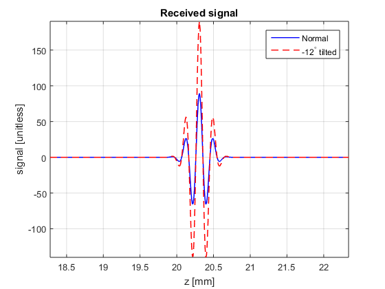
Now let us assume that the receiving transducer is tilted -12 degrees in the azimuth direction.
- Calculate the received pulse and compare it with the previous one
theta_R=atan2(P(1)-R(1),P(3)-R(3))-(-12*pi/180);
phi_R=atan2(P(2)-R(2),P(3)-R(3));
distance_R=norm(R-P,2);
directivity_R = sinc(k*a/2.*sin(theta_R).*cos(phi_R)/pi).*sinc(k*b/2.*sin(theta_R).*sin(phi_R)/pi);

% the 2-way Fresnel model for rectangular elements
s_r_tilted=directivity_T.*directivity_R.*Gamma/(4*pi*distance_T*distance_R)*cos(2*pi*f*(t-(distance_T+distance_R)/c0)).*exp(-2.77*(1.1364*(t-(distance_T+distance_R)/c0)*Deltaf).^2);

figure3 = figure('Name','background','Color',[1 1 1]);

plot(depth*1e3,s_r,'b','linewidth',1);
grid on; axis tight; hold on; box('on');
plot(depth*1e3,s_r_tilted,'r--','linewidth',1);
xlabel('z [mm]');
ylabel('signal [unitless]')
title({'Received signal'});
set(figure3,'InvertHardcopy','off');
xlim((distance_T+distance_R)/2*[0.9 1.1]*1e3);
legend('Normal','-12^\circ tilted');

- Why is the signal amplitude increased?