Physics - Tissue
This exercise tackles the simulation of biological tissue.
Related materials:
by Alfonso Rodriguez-Molares (alfonso.r.molares@ntnu.no) 19.07.2016
Contents
Tissue as a collection of points
Biological tissue can be simulated as a collection of randomly placed point scatterers. Tissue is not homogeneous. As ultrasound travels through tissue it finds minuscule fluctuations in the acoustic impedance. Part of the ultrasonic energy is scattered by those fluctuations attenuating the pulse with distance and generating a scattered wave. You can think of each of those microfluctuations as a point source at a random location. Due the superposition principle, the signal scattered by a volume of tissue can be computed as the sumation of the signals scattered in every one of those point sources,
where  denotes the convolution operation,
  denotes each of the assumed scatterers, and
  and
and  are the reflection coefficient and impulse response of the scatterer .
Some types of tissue have higher scattering intensity than other. For instance cancerous tissue is sometimes showed as a hyperechoic region (high scattering). Some kind of cysts are shown as hypoechoic regions (low scattering). That can be modelled by using different values for different regions.
We will reuse the code we wrote in the previous exercise. As before we assume the source transmits a Gaussian-modulated RF signal given by
 .
.
where the  =10 MHz, and the pulse bandwidth is
  . The system uses a sampling frequency
  = 80 MHz, and
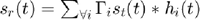
  =1540 m/s. Let us assume we have N=10000 point scatterers randomly distributed from 1 mm to 30 mm with uniform probability distribution. Assume tat =1 for all of the point scatterers.
- Can you calculate the received signal
 ?
?
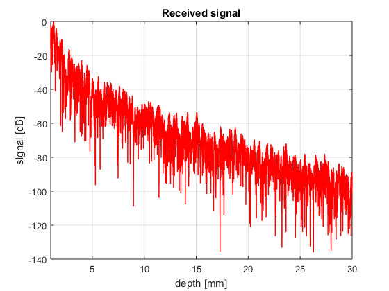
f=10e6;                     % transducer frequency [MHz]
c0=1540;                    % speed of sound [m/s]
Fs=80e6;                    % sampling frequency [Hz]
t=linspace(0,2*30e-3/c0,(2*29e-3/c0)*Fs); % time vector [s]

% calculating the trasnmittted signal
bw=0.6;         % relative bandwidth [unitless]
Deltaf=bw*f;    % bandwidth [Hz]
s_t=cos(2*pi*f*t).*exp(-2.77*(1.1364*t*Deltaf).^2); % transmitted signal

% we only show the analytical approach here
N=10000;
s_r=zeros(size(t));
for n=1:N
    r=random('unif',1e-3,30e-3);
    Gamma=1;
    s_r=s_r+Gamma/(4*pi*r)^2*cos(2*pi*f*(t-2*r/c0)).*exp(-2.77*(1.1364*(t-2*r/c0)*Deltaf).^2); % transmitted signal
end

% The envelope of the signal can be obtained via the Hilbert's transform
envelope=abs((s_r));                            % envelope of the received signal
intensity=envelope.^2;                          % intensity of the received signal
scanline=10*log10(intensity/max(intensity));    % scanline in dB
depth=c0*t/2;

figure4 = figure('Color',[1 1 1]);
plot(depth*1e3,scanline,'r','linewidth',1); grid on;
xlim([1 30]);
title({'Scanline'});
box('on');
xlabel('depth [mm]');
ylabel('signal [dB]')
title({'Received signal'});
set(figure4,'InvertHardcopy','off');
- Why the amplitude of decreases with depth?
% Due to geometrical dispersion. As the spherical wave travels more energy is distrubutted on a larger area. That is modelled by the $1/r$ factor in
% the Green's function. Absorption and scattering produce further
% attenuation but they are not included in the Green function just yet.
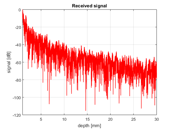
Time Gain Compensation (TGC)
In the previous section we learnt that signal amplitude decreases with depth. Obviously, we would like to compensate for that effect, so that tissue with an uniform scattering intensity has uniform brightness at all depths. We know the relation between distance and signal strength (look at Green's function again). It is possible to use that relation to design a time variable gain that compensates for dispersion.
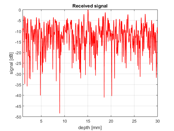
- Can you derive and apply a TGC to ?
% the attnuation predicted by the Green's function is
attenuation=1./(4*pi*depth).^2;                 % attenuation factor [unitless]

% the tgc is then simply
tgc = 1./attenuation;                           % tgc [unitless]

envelope=abs(hilbert(tgc.*s_r));                % envelope of the received signal
intensity=envelope.^2;                          % intensity of the received signal
scanline=10*log10(intensity/max(intensity));    % scanline in dB
depth=c0*t/2;

figure4 = figure('Color',[1 1 1]);
plot(depth*1e3,scanline,'r','linewidth',1); grid on;
xlim([1 30]);
title({'Scanline'});
box('on');
xlabel('depth [mm]');
ylabel('signal [dB]')
title({'Received signal'});
set(figure4,'InvertHardcopy','off');
Absorption
There are two non-linear effects that must be taken into account in ultrasound technology. One of them is the basis for harmonic imaging which we will see in the future.
The other one is sound absorption, i.e. the conversion of mechanical energy into heat. This effect is important because it affects the TGC that must be applied to have an uniform representation of the tissue scattering intensity, but also because tissue heating limits the maximum ultrasonic power that can be used on humans. We will deal with the safety limits later.
For now here is the standard model for the absorption factor
![$A = 10^{-\alpha \, r[cm] \, f_0 [MHz]/20}$](exercise_tissue_eq03741954271864701405.png)
where  is the travelled distance in cm,
  is the transmitted frequency in MHz, and
  is the absorption coefficient in dB/(cm MHz). Typical values of in the body vary from 0.5 to 0.7 dB/(cm MHz).
- Repeat the previous simulation including absorption for =0.5 dB/(cm MHz)
N=10000;
alpha=0.5;                          % absorption coefficient [dB/cm/MHz]
s_r=zeros(size(t));
for n=1:N
    r=random('unif',1e-3,30e-3);
    Gamma=1;
    s_r=s_r+10.^(-alpha.*2*r/1e-2.*f/1e6/20).*Gamma/(4*pi*r)^2*cos(2*pi*f*(t-2*r/c0)).*exp(-2.77*(1.1364*(t-2*r/c0)*Deltaf).^2); % transmitted signal
end

% The envelope of the signal can be obtained via the Hilbert's transform
envelope=abs((s_r));                     % envelope of the received signal
intensity=envelope.^2;                          % intensity of the received signal
scanline=10*log10(intensity/max(intensity));    % scanline in dB
depth=c0*t/2;

figure4 = figure('Color',[1 1 1]);
plot(depth*1e3,scanline,'r','linewidth',1); grid on;
xlim([1 30]);
title({'Scanline'});
box('on');
xlabel('depth [mm]');
ylabel('signal [dB]')
title({'Received signal'});
set(figure4,'InvertHardcopy','off');
- Can you update the TGC calculation to compensate for both geometric dispersion and absorption?
% the attnuation predicted by the Green's function is
absorption=10.^(-alpha.*2*depth/1e-2.*f/1e6/20);                 % absorption factor [unitless]

% the tgc is then simply
tgc = 1./attenuation./absorption;                           % tgc [unitless]

envelope=abs(hilbert(tgc.*s_r));                % envelope of the received signal
intensity=envelope.^2;                          % intensity of the received signal
scanline=10*log10(intensity/max(intensity));    % scanline in dB
depth=c0*t/2;

figure4 = figure('Color',[1 1 1]);
plot(depth*1e3,scanline,'r','linewidth',1);grid on;
xlim([1 30]);
title({'Scanline'});
box('on');
xlabel('depth [mm]');
ylabel('signal [dB]')
title({'Received signal'});
set(figure4,'InvertHardcopy','off');
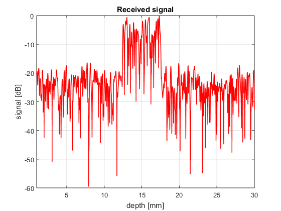
Different scattering regions
Repeat the previous simulation but this time setting two regions with different scattering intensity. For the region between ![$r\in[12.5,17.5]$](exercise_tissue_eq00035310045245284821.png) mm
mm  , and for the rest
  .
.
- Can you plot the resulting signal?
% we only show the analytical approach here
N=10000;
s_r=zeros(size(t));
for n=1:N
    r=random('unif',1e-3,30e-3);
    Gamma=0.15*ones(size(r));
    Gamma(abs(r-15e-3)<2.5e-3)=1;
    s_r=s_r+10.^(-alpha.*2*r/1e-2.*f/1e6/20).*Gamma/(4*pi*r)^2*cos(2*pi*f*(t-2*r/c0)).*exp(-2.77*(1.1364*(t-2*r/c0)*Deltaf).^2); % transmitted signal
end

envelope=abs(hilbert(tgc.*s_r));                % envelope of the received signal
intensity=envelope.^2;                          % intensity of the received signal
scanline=10*log10(intensity/max(intensity));    % scanline in dB
depth=c0*t/2;

figure4 = figure('Color',[1 1 1]);
plot(depth*1e3,scanline,'r','linewidth',1); grid on;
xlim([1 30]);
title({'Scanline'});
box('on');
xlabel('depth [mm]');
ylabel('signal [dB]')
title({'Received signal'});
set(figure4,'InvertHardcopy','off');