Physics - Scanning
This exercise summarizes the concepts see so far to create our first 2D ultrasound image!
Related materials:
by Alfonso Rodriguez-Molares (alfonso.r.molares@ntnu.no) 21.07.2016
Contents
Broadband Fresnel model for rectangular transducers
Based on the Fresnel approximation for rectangular transducer and neglecting the constant factors we can define the following LTI system to model the wave propagation for a rectangular transducer placed at  and a evaluation point placed at
  ,
,
where  is the distance between and , where

is the element directivity and

This simple model can be (and will be) used to simulate many aspects of the ultrasound imaging process.
Let us define a Gaussian-modulated RF signal
 .
.
where  = 4 MHz,
  , and
, and  =80 MHz. Consider a transducer
  =2 mm wide,
  =5 mm tall. The transducer is at the origin of coordinates with its face pointing downwards (towards positive z). Consider that a point scatterer exists at =(0,0,20) with reflection coefficient
  =1.
=1.
- Derive the two-way impulse response (transducer - reflector - transducer) and represent the received signal
% The two way impulse response is the convolution of h(t) multiplied by Gamma, with yields
%
% $h(t,\mathbf{s},\mathbf{r}) = \frac{\delta(t-2r/c_0)}{(4\pi r)^2} \, D^2(\theta,\phi)$

f=4e6;                              % transducer frequency [MHz]
Deltaf=0.6*f;                       % pulse bandwidth [MHz]
c0=1540;                            % speed of sound [m/s]
lambda=c0/f;                        % wavelength [m]
k=2*pi*f/c0;                        % wavenumber [rad/m]
Fs=80e6;                            % sampling frequency [Hz]
t=0:(1/Fs):2*40e-3/c0;              % time vector [s]
depth=t*c0/2;                       % depth vector [m]
a=2e-3;                             % element width [m]
b=5e-3;                             % element height [m]
Gamma=1;                            % reflaction coefficient [unitless]

% some geometrical variables
s=[0 0 0];                  % source position [m]
r=[0 0 20e-3];          % receive position [m]
theta=atan2(r(1)-s(1),r(3)-s(3));
phi=atan2(r(2)-s(2),r(3)-s(3));
distance=norm(s-r,2);

% the 2-way Fresnel model for rectangular elements
directivity = sinc(k*a/2.*sin(theta).*cos(phi)/pi).*sinc(k*b/2.*sin(theta).*sin(phi)/pi);
s_r=directivity.^2.*Gamma/(4*pi*distance)^2*cos(2*pi*f*(t-2*distance/c0)).*exp(-2.77*(1.1364*(t-2*distance/c0)*Deltaf).^2);

figure3 = figure('Name','background','Color',[1 1 1]);
plot(depth*1e3,s_r,'b','linewidth',1); grid on; axis tight;
box('on');
xlabel('z [mm]');
ylabel('signal [unitless]')
title({'Received signal'});
set(figure3,'InvertHardcopy','off');
xlim(distance*[0.9 1.1]*1e3);

Scanning
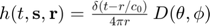
Let us place the source at (-20, 0 ,0) mm and move it along the x axis in 512 increments of 0.0781 mm.
- Calculate the signal obtained for each position of the source. Arrange the collection of signal into a 2D map (x,z). Compute the signal intensity and express it in dB. Crop anything below -60 dB
x_axis=-20e-3:0.0781e-3:20e-3;            % positions of the source

for nx=1:length(x_axis)
    s=[x_axis(nx) 0 0];                  % source position [m]
    theta=atan2(r(1)-s(1),r(3)-s(3));
    phi=atan2(r(2)-s(2),r(3)-s(3));
    distance=norm(s-r,2);

    % the 2-way Fresnel model for rectangular elements
    directivity = abs(sinc(k*a/2.*sin(theta).*cos(phi)/pi).*sinc(k*b/2.*sin(theta).*sin(phi)/pi));
    s_r(nx,:)=directivity.^2.*Gamma/(4*pi*distance)^2*cos(2*pi*f*(t-2*distance/c0)).*exp(-2.77*(1.1364*(t-2*distance/c0)*Deltaf).^2);
end

% convert to intensity values
envelope=abs(hilbert(s_r.'));
envelope_dB=20*log10(envelope./max(envelope(:)));

figure3 = figure('Name','background','Color',[1 1 1]);
imagesc(x_axis*1e3,depth*1e3,envelope_dB); axis tight equal;
box('on');
xlabel('x [mm]');
ylabel('z [mm]')
title({'Received signal'});
set(figure3,'InvertHardcopy','off');
caxis([-60 0]); colorbar; colormap gray;
- Can you identify the main lobe? And the sidelobes?
% Yes.
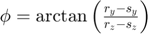
- Check what happens when you change the width of the transducer.
a=20e-3;                    % transducer width [m]

for nx=1:length(x_axis)
    s=[x_axis(nx) 0 0];                  % source position [m]
    theta=atan2(r(1)-s(1),r(3)-s(3));
    phi=atan2(r(2)-s(2),r(3)-s(3));
    distance=norm(s-r,2);

    % the 2-way Fresnel model for rectangular elements
    directivity = abs(sinc(k*a/2.*sin(theta).*cos(phi)/pi).*sinc(k*b/2.*sin(theta).*sin(phi)/pi));
    s_r(nx,:)=directivity.^2.*Gamma/(4*pi*distance)^2*cos(2*pi*f*(t-2*distance/c0)).*exp(-2.77*(1.1364*(t-2*distance/c0)*Deltaf).^2);
end

% convert to intensity values
envelope=abs(hilbert(s_r.'));
envelope_dB=20*log10(envelope./max(envelope(:)));

figure3 = figure('Name','background','Color',[1 1 1]);
imagesc(x_axis*1e3,depth*1e3,envelope_dB); axis tight equal;
box('on');
xlabel('x [mm]');
ylabel('z [mm]')
title({'Received signal'});
set(figure3,'InvertHardcopy','off');
caxis([-60 0]); colorbar; colormap gray;
- What is the relation between the transducer width and the lateral resolution? No need to derive it, just check the general trend
% Lateral resolution increases with the transducer width.
The Fresnel approximation is only valid for points in the far field, which starts beyond

- Check if the previous simulations were correct
% case 1
a=2e-3;
z_far=a^2/4/lambda
if(20e-3>z_far) disp('Yes!'); else disp('Nope'); end

% case 2
a=20e-3;
z_far=a^2/4/lambda
if(20e-3>z_far) disp('Yes!'); else disp('Nope'); end
z_far =

    0.0026

Yes!

z_far =

    0.2597

Nope