Physics - Plannar sources
This exercise introduces some typical models for plane transducers and some important features of ultrasonic beams.
Related materials:
by Alfonso Rodriguez-Molares (alfonso.r.molares@ntnu.no) 19.07.2016
Contents
The problem with points
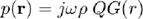
In the previous exercises we couldn't locate a point scatterer in space using a single point source. The sound pressure generated by a point source (monopole) vibrating harmonically is given by,
where  is the volume velocity (not very important for you right now) and
  is the Green's function in the frequency domain

where  is the wavenumber and
  is the distance between the source and the evaluation point.
Let's assume a point source is at the origin of coordinates, vibrating continuously at 2 MHz frequency with = 1e-5 m3/s. Assume the speed of sound in the medium is 1540 m/s and its density is 1020 kg/m3. Define a grid of points within ![$x\in [-10, 10]$](exercise_plannar_sources_eq16101892564771254225.png) mm and
mm and ![$z \in [1, 60]$](exercise_plannar_sources_eq05056913011527554699.png) mm.
mm.
- Calculate and plot sound pressure level
% some constants
c0 = 1540;                                    % sound speed [m/s]
rho = 1020;                                   % density [kg/m3]
Q = 1.0e-5;                                   % volume velocity [m3/s]
f = 2e6;                                      % frequency [Hz]
w = 2*pi*f;                                   % angular frequency [rad/s]
k = w/c0;                                     % wavenumber [rad/m]
t = linspace(0,1/f,10);                       % time vector [s]

% we select the zone where we will evaluate the Green function
x_axis = linspace(-10e-3,10e-3,4*20);          % x axis [m]
z_axis = linspace(1e-3,60e-3,4*60);            % z axis [m]
[X Z] = meshgrid(x_axis,z_axis);              % x and z coordinates in grid form [m]
Y = zeros(size(X));                           % y coordinates in grid form [m]
R=sqrt(X.^2+Z.^2);                            % distance form the evaluation point to the source (at origin)

% the magnitude numerator, thus the magnitude of the Green's
figure1 = figure('Name','background','Color',[1 1 1]);
set(gcf,'Position',[  235   -73   771   775]);
for n=1:length(t)

    % formula
    p=j*w*rho*Q*exp(j*(w*t(n)-k*R))./(4*pi*R);

    subplot(1,2,1);
    imagesc(x_axis*1e3,z_axis*1e3,real(p)/1e6); axis equal tight;
    colorbar;
    xlabel('x [mm]');
    ylabel('z [mm]');
    title('Sound pressure [MPa]');
    set(figure1,'InvertHardcopy','off');
    caxis([-max(abs(p(:))) max(abs(p(:)))]/1e6);

    subplot(1,2,2);
    imagesc(x_axis*1e3,z_axis*1e3,20*log10(abs(p)/1e-6)); axis equal tight;
    colorbar; %caxis([-60 0]);
    xlabel('x [mm]');
    ylabel('z [mm]');
    title('Sound Pressure Level [dB]');
    set(figure1,'InvertHardcopy','off');

    pause(0.1)
    drawnow;
end
- Why is not possible to locate scatterers with a single point source?
% Because point sources/receivers are omnidirectional. The energy is sent evernly in
% all directions so that it is impossible to distiguish where the energy
% goes and comes from.
Planar sources
A radiating surface sends energy in a specific direction. One of the simplest, yet accurate, descriptions of radiating surfaces is the Rayleigh integral
where  is the evaluation point,
  is a point in the radiating surface,
  is the distance between
  and
and  ,
, ![$v_0 [\textmd{m/s}]$](exercise_plannar_sources_eq02666893980905135443.png) is the velocity of the surface,
is the velocity of the surface, ![$\omega = 2 \pi f~[\textmd{rad/s}]$](exercise_plannar_sources_eq07915557495206436558.png) is the angular frequency, and
is the angular frequency, and ![$k=\omega/c0~[\textmd{rad/m}]$](exercise_plannar_sources_eq18197870731386847789.png) is the wavenumber.
is the wavenumber.
We can visualize the Rayleigh integral using Huygens' principle. Imagine a zillion of point sources placed on the radiating surface, all vibrating in synchrony with velocity  , and interfering with each other positive and destructively. Rayleigh's integral makes use the same approach we applied to simulate speckle in a previous exercise. As per the superposition principle, adding the contribution of each infinitesimal source, we obtain the sound pressure at .
Let assume we have a rectangular transducer, 5 mm wide and 5 mm tall. Said transducer vibrates continuously (CW) at a frequency of 2 MHz and with a velocity of 1 m/s. The element is centered at the origin of coordinates in a domain with 1540 m/s sound speed and 1020 kg/m3 density. Use the same grid as in the previous section.
- Represent the sound pressure level produced by the transducer?
% some constants
v0= 1;                                       % velocity at the probe surface [m/s]
a= 5e-3;                                     % transducer width [m]
b= 5e-3;                                     % trasnducer height [m]

% simulation parameters
pixels=numel(X);                             % number of evaluation points
N=10000;                                     % number of sources that we will use in the simulation
chunksize=1000;                              % size of the chunk that we will calculate in parallel
chunks=ceil(N/chunksize);                    % number of chunks to calculate

% loop
sum_green=zeros(1,pixels);                         % map we want to create
for n=1:(N/chunksize)
    disp(sprintf('Computing chunk %d of %d',n,chunks));

    % we set random source location within the transducer surface
    s = [random('unif',-a/2,a/2,chunksize,1) random('unif',-b/2,b/2,chunksize,1) zeros(chunksize,1)];

    % compute distance from all sources to all pixels
    R = sqrt((s(:,1)*ones(1,pixels)-ones(chunksize,1)*X(:).').^2+...
        (s(:,2).^2*ones(1,pixels))+...
        (ones(chunksize,1)*(Z(:).^2).'));

    % compute Green function and we add the contribution from all sources and multiply by the constants
    sum_green=sum_green+sum(exp(-1i*k*R)./(4*pi*R),1);
end

% insert the constants
p=j*w*rho*2*v0*sum_green*(a*b/(chunks*chunksize));

% reshape results so that it becomes a matrix
p=reshape(p,[size(X,1) size(X,2)]);

% the magnitude numerator, thus the magnitude of the Green's
figure2 = figure('Name','background','Color',[1 1 1]);
set(gcf,'Position',[  235   -73   771   775]);
for n=1:length(t)

    % we show the map
    subplot(1,2,1);
    imagesc(x_axis*1e3,z_axis*1e3,real(p*exp(j*w*t(n)))/1e6); axis equal tight;
    colorbar;
    xlabel('x [mm]');
    ylabel('z [mm]');
    title('Sound pressure [MPa]');
    set(figure2,'InvertHardcopy','off');
    caxis([-max(abs(p(:))) max(abs(p(:)))]/1e6);

    % we show the map
    subplot(1,2,2);
    imagesc(x_axis*1e3,z_axis*1e3,20*log10(abs(p)/1e-6)); axis equal tight;
    colorbar; %caxis([-60 0]);
    xlabel('x [mm]');
    ylabel('z [mm]');
    title('Sound Pressure Level [dB]');
    set(figure2,'InvertHardcopy','off');

    drawnow();
end
Computing chunk 1 of 10
Computing chunk 2 of 10
Computing chunk 3 of 10
Computing chunk 4 of 10
Computing chunk 5 of 10
Computing chunk 6 of 10
Computing chunk 7 of 10
Computing chunk 8 of 10
Computing chunk 9 of 10
Computing chunk 10 of 10
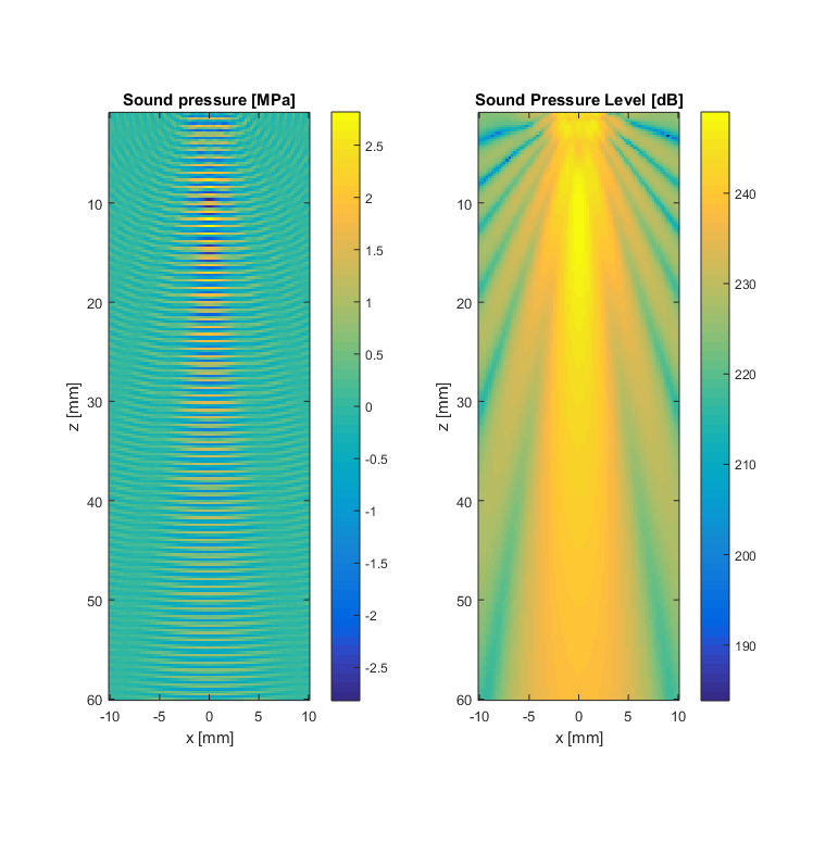
- Can you identify the main lobe and the side lobes? Where is the near field?
% Yes. I can.
- Why do we have side lobes? Why don't we see a single straight line in front of the transducer?
% Due to the diffraction and the transducer edges. The transition between
% a region with point sources and a region without makes a complex wave
% pattern. At some points in space the sources at the edge will interfere
% constructively and sidelobes will arise. In some other points they will
% interfere destructively and no sidelobes are seen.
%
% Apodization can be used to reduce the energy of the sidelobes, but more
% on that when we get to beamforming.
- Approximately, how many point sources do you need to get a good approximation?
% That depend on the transducer size, frequency, and the location of te
% evaluation points. The larger the transducer, the larger the frequency,
% and the closer the location, the larger number of sources we need. For this
% example, N=5000 is enough to get a fair approximation of the main lobe.
% To approximate the sidelobes, however, N=10000 is needed or even higher.
The Fresnel model for rectangular transducers
The numerical integration of Rayleigh's integral is accurate, as long as you use a high enough number of point sources (ridiculously high). Rayleigh is not a good option for fast simulation of beam profiles.
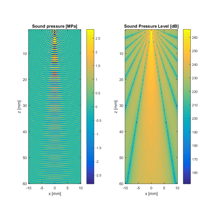
Under the paraxial approximation, for rectangular transducers, and in the far-field, the Rayleigh integral can be further simplified, yielding the Fresnel expression

where  is the element width,
  is the element height, is the distance between the transducer and the evaluation point, and
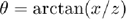
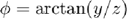
are the incidence angles in azimuth and elevation direction, respectively, between the transducer and the point .
- epresent the sound pressure level using the Fresnel approximation?
% some gemetrical variables
THETA=atan2(X,Z);
PHI=atan2(Y,Z);
R=sqrt(X.^2+Y.^2+Z.^2);

% the fresnel model
p_theory = j*w*rho*a*b*v0.*exp(-j*k*R)./2/pi./R .*sinc(k*a/2.*sin(THETA).*cos(PHI)/pi).*sinc(k*b/2.*sin(THETA).*sin(PHI)/pi);

% the magnitude numerator, thus the magnitude of the Green's
figure2 = figure('Name','background','Color',[1 1 1]);
set(gcf,'Position',[  235   -73   771   775]);
for n=1:length(t)

    % we show the map
    subplot(1,2,1);
    imagesc(x_axis*1e3,z_axis*1e3,real(p_theory*exp(j*w*t(n)))/1e6); axis equal tight;
    colorbar;
    xlabel('x [mm]');
    ylabel('z [mm]');
    title('Sound pressure [MPa]');
    set(figure2,'InvertHardcopy','off');
    caxis([-max(abs(p(:))) max(abs(p(:)))]/1e6);

    % we show the map
    subplot(1,2,2);
    imagesc(x_axis*1e3,z_axis*1e3,20*log10(abs(p_theory)/1e-6)); axis equal tight;
    colorbar; %caxis([-60 0]);
    xlabel('x [mm]');
    ylabel('z [mm]');
    title('Sound Pressure Level [dB]');
    set(figure2,'InvertHardcopy','off');

    drawnow();
end
Main axis
- Compare the sound pressure level on the beam axis for both models: Rayleigh and Fresnel
figure;
plot(z_axis*1e3,20*log10(abs(p(:,numel(x_axis)/2))/1e-6)); hold on; grid on;
plot(z_axis*1e3,20*log10(abs(p_theory(:,numel(x_axis)/2))/1e-6));
xlabel('z [mm]');
ylabel('Sound Pressure Level (dB)');
legend('Rayleigh integral','Fresnel approximation');
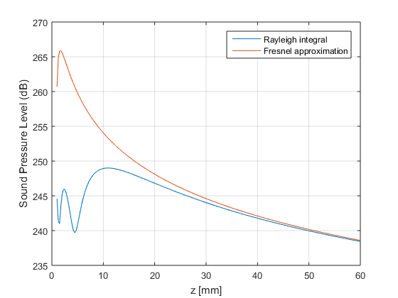
- What differences do you see between the results obtained with the Rayleigh's integral and the Fresnel approximation?
% The Fresnel approximation is only valid in the far field, hence it fails
% to model the natural focus of the transducer, and the near field.