Physics - Circular transducers and more on the main axis
We keep learning on beam profile characteristics and how they condition ultrasonics imaging, this time using circular transducers.
Related materials:
by Alfonso Rodriguez-Molares (alfonso.r.molares@ntnu.no) 20.07.2016
Contents
Circular transducers
In order to get a clearer understanding of what happens right in front of the transducer we are going to forget about sidelobes and explore the acoustic field along the beam axis. To keep it simple we will now concentrate on circular transducers.
Let assume we have a circular transducer of 3 mm diameter. Said transducer vibrates in continuous mode at a frequency of 8 MHz and with a 1e-3 m/s velocity . The element is centered at the origin of coordinates in a domain with 1540 m/s sound speed and 1020 kg/m3 density.
- Can you calculate the acoustic field along the z-axis (from 1 to 40 mm) using the Rayleigh integral?
% some constants
f= 8e6;                                      % frequency [Hz]
c0= 1540;                                    % speed of sound [m/s]
rho= 1020;                                   % density [kg/m2]
w= 2*pi*f;                                   % angular frequency [rad/s]
k= w/c0;                                     % wavenumber [rad/m]
v0= 1e-3;                                    % velocity at the probe surface [m/s]
a= 3e-3;                                     % transducer diameter [m]

% simulation parameters
z_axis=linspace(1e-3,40e-3,256);             % z-axis [m]
pixels=numel(z_axis);                        % number of evaluation points
N=80000;                                     % number of sources that we will use in the simulation
chunksize=10000;                              % size of the chunk that we will calculate in parallel
chunks=ceil(N/chunksize);                    % number of chunks to calculate

% loop
p=zeros(1,pixels);                   % signal we want to create
den=0;
for n=1:(N/chunksize)
    disp(sprintf('Computing chunk %d of %d',n,chunks));

    % we set random source location within the transducer surface
    s_r=random('unif',0,a/2,chunksize,1);
    s_theta=random('unif',0,2*pi,chunksize,1);

    s = [s_r.*cos(s_theta) s_r.*sin(s_theta) zeros(chunksize,1)];

    % compute distance from all sources to all pixels
    R = sqrt(s(:,1).^2*ones(1,pixels)+...
            (s(:,2).^2*ones(1,pixels))+...
            (ones(chunksize,1)*(z_axis.^2)));

    % compute Green function
    green = (s_r*ones(1,pixels)).*exp(-1i*k*R)./(4*pi*R);                     % green function handle

    % Careful about forgetting the Jacobian! If you use the function below
    % the integration will be wrong. Alternatively can you do the
    % integration in cardinal coordinates and only use points inside the
    % circle.
    % green = exp(-1i*k*R)./(4*pi*R);                     % green function handle

    % we add the contribution from all sources and multiply by the constants
    p=p+sum(green,1);
end

% insert the constants
p=j*w*rho* 2*v0* p* (pi*a/(chunks*chunksize));

% we show the beam axis
figure4 = figure('Name','background','Color',[1 1 1]);
plot(z_axis*1e3,20*log10(abs(p)/1e-6)); axis tight; hold on; grid on;
xlabel('z [mm]');
ylabel('Sound Pressure Level [dB]');
set(figure4,'InvertHardcopy','off');
Computing chunk 1 of 8
Computing chunk 2 of 8
Computing chunk 3 of 8
Computing chunk 4 of 8
Computing chunk 5 of 8
Computing chunk 6 of 8
Computing chunk 7 of 8
Computing chunk 8 of 8
An exact formula for the on-axis pressure
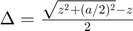
For this specific case an analytical formula can be derived, without any assumptions:

where,
- Can you compare the numerical result obtained in the previous exercise with this analytical formula?
% compute the analytical
Delta=0.5*(sqrt(z_axis.^2+(a/2)^2)-z_axis);
p_ana=j*rho*c0*2*v0*exp(-j*k*(z_axis+Delta)).*sin(k*Delta);

% we show the plot
figure4 = figure('Name','background','Color',[1 1 1]);
plot(z_axis*1e3,20*log10(abs(p)/1e-6)); axis tight; hold on; grid on;
plot(z_axis*1e3,20*log10(abs(p_ana)/1e-6),'r--');
xlabel('z [mm]');
ylabel('Sound Pressure Level [dB]');
set(figure4,'InvertHardcopy','off');
legend('Numerical','Analytic');
- Can you identify where the natural focus of the beam is? Using the analytical formula, can you derive an expression for the location of the natural focus?
% The natural focus is the farthest maximum from the aperture. By
% inspecting the formula we see that this maximum correspond to
%
% k*Delta=pi/2.
%
% Inserting the definition of Delta and operating we obtain:
%
% Delta = pi/2/k = c/f/4 = lambda/4
%
% sqrt(z^2+(a/2)^2) - z = lambda/2
%
% z^2 + (a/2)^2 = (lambda/2)^2 + lambda*z + z^2
%
% z = (a/2)^2/lambda - lambda/4
%
% So:

lambda = c0/f;                      % wavelength [m]
z_max = (a/2)^2/lambda - lambda/4   % position of the natural focus [m]

% we show the plot
figure4 = figure('Name','background','Color',[1 1 1]);
plot(z_axis*1e3,20*log10(abs(p)/1e-6)); axis tight; hold on; grid on;
plot(z_axis*1e3,20*log10(abs(p_ana)/1e-6),'r--');
plot(z_max*1e3*[1 1],[min(20*log10(abs(p_ana)/1e-6)) max(20*log10(abs(p_ana)/1e-6))],'g--');
plot(z_max*1e3,max(20*log10(abs(p_ana)/1e-6)),'go');
xlabel('z [mm]');
ylabel('Intensity [dB]');
title('Transducer beam axis');
set(figure4,'InvertHardcopy','off');
legend('Numerical','Analytic','Natural focus');
z_max =

    0.0116
Fresnel approximation for the on-axis pressure
This is the Fresnel approximation for the on axis pressure

- Plot the three expressions
% compute the analytical
p_far=j*w*rho* (pi*(a/2)^2) * 2*v0*  exp(-j*k*z_axis)/4/pi./z_axis;

% we show the plot
figure4 = figure('Name','background','Color',[1 1 1]);
plot(z_axis*1e3,20*log10(abs(p)/1e-6)); axis tight; hold on; grid on;
plot(z_axis*1e3,20*log10(abs(p_ana)/1e-6),'r--');
plot(z_axis*1e3,20*log10(abs(p_far)/1e-6),'g-.');
xlabel('z [mm]');
ylabel('Sound Pressure Level [dB]');
set(figure4,'InvertHardcopy','off');
legend('Numerical','Analytic','Fresnel');