Physics - Linear Time Invariant Systems

This exercise shows how ultrasonic wave propagation can be model as a linear and time invariant (LTI) system.

Related materials:

by Alfonso Rodriguez-Molares (alfonso.r.molares@ntnu.no) 18.07.2016

Wave propagation as a LTI system
Envelope
Decibels
Depth axis
Axial resolution

Wave propagation as a LTI system

Under free-field condition it is possible to model the one-way wave propagation between point $\mathbf{s}$ and point $\mathbf{r}$ as a LTI system

where

$G(r,t)= \frac{\delta(t-r/c_0)}{4 \pi r}$

is the Green's function, $t$ is the time vector, and $r=||\mathbf{r} - \mathbf{s}||$ is the distance between $\mathbf{s}$ and $\mathbf{r}$ .

The Green's function indicates that the signal received at $\mathbf{r}$ from the source $\mathbf{s}$ is just a delayed and attenuated copy of the transmitted signal.

Once the signal arrives at $\mathbf{r}$ , and assuming there is point reflector at $\mathbf{r}$ with reflection coefficient $\Gamma$ , the signal will be scattered back to the source. The back propagation from $\mathbf{r}$ to $\mathbf{s}$ can also be modelled with the Green's function.

Derive the 2-way impulse response from a source at $\mathbf{s}$ to $\mathbf{r}$ and back.

% The 2-way impulse response will be the convolution of $G(t,r)$ and
% $G(t,r)$ multiplied by the reflection coefficient $Gamma$, i.e.
%
% $h(t,r)= \Gamma \frac{\delta(t-2 r/c_0)}{8 \pi^2 r^2} $

The source transmits a Gaussian-modulated RF signal given by

$s_t(t) = \cos \left(2\pi f t\right) e^{-2.77 \left(1.1364 \, t \, \Delta f\right)^2}$ .

where the transmit frequency $f$ =10 MHz, and the pulse bandwidth is $\Delta f=0.6 f$ . Assuming that the system uses a sampling frequency $F_s$ = 80 MHz, that $c_0$ =1540 m/s, and that a target with $\Gamma$ = 1 is placed 23.7 mm away from the source-receiver,

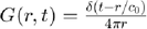
Compute and plot the signal received back at the source

% We need to select a time vector long enough so that we cover the moment
% the reflected signal arrives. Also, as $s_t(t)$ is a bandpass pulse and
% symetric respect to $t=0$ we must expand our time vector a bit to cover
% the transmitted and received pulse completely. Three cycles should be
% enough for a 60% badnwidth pulse.
f=10e6;                     % transducer frequency [MHz]
c0=1540;                    % speed of sound [m/s]
r=23.7e-3;                  % distance to the target [m]
Fs=80e6;                    % sampling frequency [Hz]
offset=3/f;                 % offset applied to cover the pulse completely
t=linspace(-offset,offset+2*30e-3/c0,(2*30e-3/c0+2*offset)*Fs); % time vector [s]

% calculating the trasnmittted signal
bw=0.6;         % relative bandwidth [unitless]
Deltaf=bw*f;    % bandwidth [Hz]
s_t=cos(2*pi*f*t).*exp(-2.77*(1.1364*t*Deltaf).^2); % transmitted signal

% The received signal is given by convolution of the transmitted signal
% $s_t(t)$ and the impulse response $h(t)$
%
% $s_r(t) = s_t(t) * h_n(t)$
%
% There are several waves of simulating this, some more accurate than the
% other.

% Solution 1 ------------------------------------------------------------
% The most intuitive is perhaps to build the impulse response $h(t)$ as a
% digital delta for at the location closest to t=2r/c and convolve it with
% s_t(t):

% estimating the position of the delta by the nearest neighbor
% approximation
[dummy n]=min(abs(t-2*r/c0));

% building the impulse response
Gamma=1;                    % reflection coefficient [unitless]
h=zeros(size(t));
h(n)=Gamma/(4*pi*r)^2;

% computing the receive signal as the convolution
s_r=conv(s_t,h);

% but convolution redefines the time axis, so we have to do the same
t_conv=linspace(2*t(1),2*t(end),length(s_r));

figure2 = figure('Name','background','Color',[1 1 1]);
plot(t_conv*1e6,s_r,'b','linewidth',1); grid on; axis tight
box('on');
xlabel('t [\mus]');
ylabel('signal [unitless]')
title({'Received signal'});
set(figure2,'InvertHardcopy','off');
xlim(2*r/c0*[0.9 1.1]*1e6);

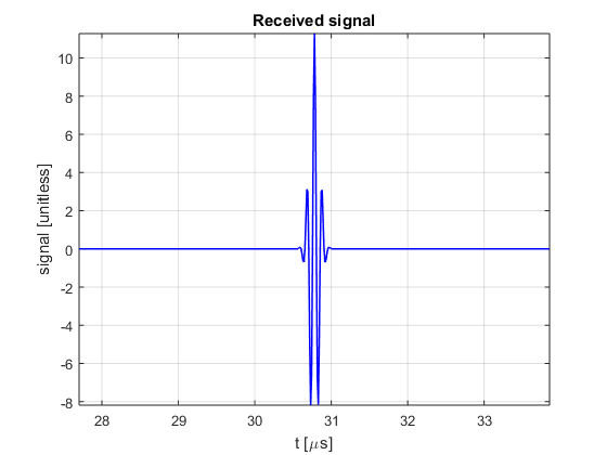
% Solution 2 ------------------------------------------------------------
% A more efficient (and elegant) solution is to calculate the convolution
% analitically and build the receive signal directly. Just by:

Gamma=1;                    % reflection coefficient [unitless]

s_r=Gamma/(4*pi*r)^2*cos(2*pi*f*(t-2*r/c0)).*exp(-2.77*(1.1364*(t-2*r/c0)*Deltaf).^2); % transmitted signal

figure3 = figure('Name','background','Color',[1 1 1]);
plot(t*1e6,s_r,'b','linewidth',1); grid on; axis tight;
box('on');
xlabel('t [\mus]');
ylabel('signal [unitless]')
title({'Received signal'});
set(figure3,'InvertHardcopy','off');
xlim(2*r/c0*[0.9 1.1]*1e6);

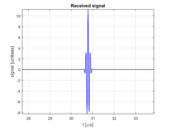
Envelope

In ultrasound images we do not show RF frequency signals, but amplitude signals where pixel brightness is related to the signal envelope. There are several way of computing the envelope.

Choose one and plot the envelope of the received signal .

% There are several ways of computing the envelope. One of the simplest, is
% by the hilbert trasform, providing that the signal sampling fulfills the
% Nyquish criterium

envelope=abs(hilbert(s_r));

figure3 = figure('Name','background','Color',[1 1 1]);
plot(t*1e6,envelope,'b','linewidth',1);grid on; axis tight;
box('on');
xlabel('t [\mus]');
ylabel('signal amplitude [unitless]')
title({'Received signal'});
set(figure3,'InvertHardcopy','off');
xlim(2*r/c0*[0.9 1.1]*1e6);

Decibels

Acoustic signals can have a very large range of values, comprising several orders of magnitud. To facilitate visualization we apply some compression of the signal envelope. Most systems do that by representing the amplitude of ultrasonic signals in dB. To avoid having arbitrarily large numbers we normalize the signal by the maximum intensity, so that it becomes 0 dB.

Plot the envelope of in dB.

% Easy peasy
envelope_dB=20*log10(envelope./max(envelope(:)));

figure3 = figure('Color',[1 1 1]);
plot(t*1e6,envelope_dB,'b','linewidth',1); grid on; axis tight;
box('on');
xlabel('t [\mus]');
ylabel('signal amplitude [unitless]')
title({'Received signal'});
set(figure3,'InvertHardcopy','off');
xlim(2*r/c0*[0.9 1.1]*1e6);

Depth axis

Ultrasound signal are represented in terms of the distance (in mm), rather than time.

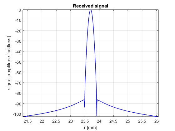
Plot the envelope in dB versus distance?

% compute z_axis
r_axis=c0*t/2;

figure3 = figure('Color',[1 1 1]);
plot(r_axis*1e3,envelope_dB,'b','linewidth',1); grid on; axis tight;
box('on');
xlabel('r [mm]');
ylabel('signal amplitude [unitless]')
title({'Received signal'});
set(figure3,'InvertHardcopy','off');
xlim(r*[0.9 1.1]*1e3);

Axial resolution

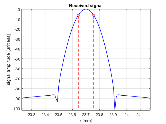
The axial resolution tells us how well the system can resolve two targets placed at almost the same depth (resolution in the z direction). Resolution is normally estimated by means of the pulse full width half maximum (FWHM), i.e. twice the -6dB pulse width.

Calculate the FWHM of

% we estimate the pulse location
[peak_value peak_index]=max(envelope_dB);

% we get only a portion of the pulse
width_index=2/f*Fs;
r_beam=r_axis(peak_index:peak_index+width_index);
e_beam=envelope_dB(peak_index:peak_index+width_index);

% we obtain the -6dB point by interpolation
r_6dB=interp1(e_beam,r_beam,-6,'linear');

% FWHM
FWHM= 2*(r_6dB-r_axis(peak_index))

% we plot it
figure3 = figure('Color',[1 1 1]);
plot(r_axis*1e3,envelope_dB,'b','linewidth',1); grid on; axis tight; hold on;
plot((r+FWHM/2)*1e3,-6,'ro');
plot((r-FWHM/2)*1e3,-6,'ro');
plot([r-FWHM/2 r+FWHM/2]*1e3,-6*[1 1],'r--');
plot((r+FWHM/2)*[1 1]*1e3,[-100 -6],'r--');
plot((r-FWHM/2)*[1 1]*1e3,[-100 -6],'r--');
box('on');
xlabel('r [mm]');
ylabel('signal amplitude [unitless]')
title({'Received signal'});
set(figure3,'InvertHardcopy','off');
xlim(r*[0.98 1.02]*1e3);

FWHM =

   1.0974e-04

Which factors determine the axial resolution of the system?

% The pulse duration which, with the formulation introduced here, depends
% on the bandwidth of the transmitted pulse. This bandwidth depends in
% turns on the bandwidth of the transducer and the bandwidth of a
% excitation signal that often contains several cycles of the transmit
% frequency.