System Architecture - Frontend

In this problem we review some of the concepts we have seen in previous sessions and follow on the impact that they have on the Front-End Components. You should have a look at the chapter written by Bruner first.

Related materials:

by Lasse Løvstakken (lasse.lovstakken@ntnu.no) and Alfonso Rodriguez-Molares (alfonso.r.molaes@ntnu.no) 10.11.2016

Tasks of the Front End
Data transfer
Number of beams
Expanding aperture
Size of beamforming filters

Tasks of the Front End

What functions are done in the Front End?

% Transmit: Pulse generator and amplifier, transmit delay generator, pulse trigger, multiplexer (optional)
% Receive: Protection circuit, low-noise amplifier, depth-dependent amplifier, anti-aliasing filter, analog-to-digital converter, beamformer including receive delay generation and apodization, multiplexer (optional)

Synchronization is fundamental for ultrasound imaging. Make a list of different issues when it comes to synchronization.

% Tx pulse trigger is the reference for the receive line. Receive is
% started a certain time after tx trig. Range gating is done assuming a
% fixed speed of sound, c=1540m/s. Pulses are fired at a given pulse
% repetition frequency (PRF) determined by the image depth (pulse-echo).
% There is also a frame trigger pulse which indicates the start of a new
% sequence of pulses. Timing is especially important in Doppler processing,
% where the phase information at the center frequency is used to estimate
% motion. The PRF must be constant.

Data transfer

Assume that we want to make 2D tissue imaging with a phased array. The system has 128 channels, the signals are digitized (A/D-converted) with 12 bits resolution with a sample rate of 40 MSamples/s. Assume we utilize all available channels and that all data is transferred to a digital processing unit.

What is the datarate into such processing unit?

channels= 128;                      % channels
Fs=40e6;                            % sampling frequency [Hz]
resolution=12;                      % sample resolution [bit]
datarate = channels*Fs*resolution;  % datarate [bps]

disp(sprintf('The needed datarate is %0.2f GB/s',datarate/1024^3/8));

The needed datarate is 7.15 GB/s

Number of beams

We use a 90° opening angle, and a transmit focus depth of 70 mm. The probe aperture is 20 mm. The probe central frequency is 3 MHz. Assume the beam width $BW$ can be approximated by $2\lambda F$ (i.e. two times the wavenumber times the F-number). The beam overlap is then defined as:

$\textmd{overlap} (\%) = \left( 1 - \frac{dx}{BW} \right)\cdot 100$

A 50% beam overlap is used at focal depth. The medium speed of sound is 1540 m/s, as usual.

Compute the minimum number of beams needed to cover the desired field-of-view

f=3e6;                      % central frequency [Hz]
c0=1540;                    % speed of sound [m/s]
lambda=c0/f;                % wavenumber [m]
focal_depth=70e-3;          % focal depth [m]
aperture=20e-3;             % probe aperture [m]
pitch=aperture/channels;    % pitch
F=focal_depth/aperture;     % F-number
BW=2*lambda*F;              % beam width [m]
beam_overlap=0.5;           % beam overlap []

dx=BW*(1-beam_overlap);     % distance between adjacent beams at the focal depth [m]
dtheta=atan(dx/focal_depth);% angle between adjacent beams
N_beams=ceil(pi/2/dtheta);  % number of beams

disp(sprintf('We need %d beams',N_beams));

We need 62 beams

Expanding aperture

We will use expanding aperture and we are considering to make 3 different modes available for the user with F-numbers 1.5, 3.5 and 7.

Compute the maximum depth we can attain while keeping those F-numbers

F_number=[1.5 3.5 7.5];     % possible F-numbers
z_max=F_number*aperture;    % corresponding maximum depths [m]

disp(sprintf('The maximum depth for F=[%0.1f, %0.1f, %0.1f] is z_max=F=[%0.0f, %0.0f, %0.0f] mm',F_number,z_max*1e3));

The maximum depth for F=[1.5, 3.5, 7.5] is z_max=F=[30, 70, 150] mm

Defining the lateral resolution as half the beam width (BM), compute the lateral resolution (before the maximum depth) for each of these modes

BW=2*F_number*lambda;       % beam width [m]
lateral_resolution=BW/2;    % lateral resolution [m]

disp(sprintf('The lateral resolution is [%0.1f, %0.1f, %0.1f] mm',lateral_resolution*1e3));

The lateral resolution is [0.8, 1.8, 3.8] mm

For each respective mode, after the maximum depth, Will the F-number be higher or lower?

And hence, will then the resolution be higher of lower?

For each mode compute the axial resolution at 30 mm

zc=30e-3;
aperture_at=min([zc./F_number; aperture*ones(1,3)]);  % aperture [m]
F_number_at=zc./aperture_at;                          % F-number
BW_at=2*F_number_at*lambda;                           % beam width [m]
lateral_resolution_at=BW_at/2;                        % lateral resolution [m]

disp(sprintf('The lateral resolution at %0.0f mm is [%0.1f, %0.1f, %0.1f] mm',zc*1e3,lateral_resolution_at*1e3));

The lateral resolution at 30 mm is [0.8, 1.8, 3.8] mm

For each mode compute the axial resolution at 100 mm

zc=100e-3;
aperture_at=min([zc./F_number; aperture*ones(1,3)]);  % aperture [m]
F_number_at=zc./aperture_at;                          % F-number
BW_at=2*F_number_at*lambda;                           % beam width [m]
lateral_resolution_at=BW_at/2;                        % lateral resolution [m]

disp(sprintf('The lateral resolution at %0.0f mm is [%0.1f, %0.1f, %0.1f] mm',zc*1e3,lateral_resolution_at*1e3));

The lateral resolution at 100 mm is [2.6, 2.6, 3.8] mm

For each mode compute the axial resolution at 150 mm

zc=150e-3;
aperture_at=min([zc./F_number; aperture*ones(1,3)]);  % aperture [m]
F_number_at=zc./aperture_at;                          % F-number
BW_at=2*F_number_at*lambda;                           % beam width [m]
lateral_resolution_at=BW_at/2;                        % lateral resolution [m]

disp(sprintf('The lateral resolution at 150 mm is [%0.1f, %0.1f, %0.1f] mm',lateral_resolution_at*1e3));

The lateral resolution at 150 mm is [3.8, 3.8, 3.8] mm

Size of beamforming filters

We implement the receive beamforming delays with FIR-filters, after A/D conversion. To achieve greater the signal is upsampled 4 times before the delay step.

Using expanding aperture and a F-number of 3.5, What would be the minimum length (in samples) of these FIR filters? For simplicity, consider the case without steering (x=0).

% For the non steering case the maximum delay will be given by the
% difference between the length of the path from the edge of the aperture (E) to the focal
% point (F), and the length of the path from the origin (O) and the focal
% point.
%
% delay=(dist(E,F)-dist(O,F))/c0;
%
% where E = [z/F/2, 0]
%       F = [0, z]
%       O = [0, 0]
%
% Inserting those points into the equation we get:
%
% delay=(sqrt(z^2+(z/(2F))^2)-z)/c0
%
% however z/(2F) cannot be larger than A/2

% we represent the maximum delay against depth up to 15 cm
z=linspace(0,150e-3,100);                   % depth vector [m]
xe=min([z/2/F ; aperture/2*ones(1,100)]);   % expanding aperture semiwidth [m]
F=3.5;                                      % F-number
delay=(sqrt(z.^2+(xe).^2)-z)/c0;                % delay [s]

figure;
plot(z*1e3,delay*1e6); hold on; grid on;
ylabel('Maximum delay [\mus]');
xlabel('Depth [mm]');

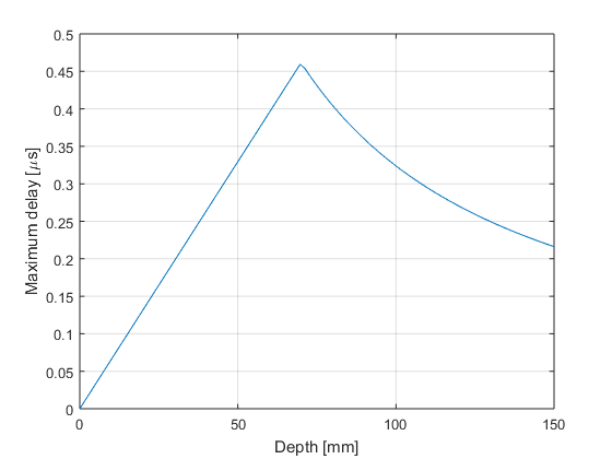
% Therefore the maximum delay will be at z=F*aperture

max_delay=aperture/c0*(sqrt(F^2+1/4)-F);

figure;
plot(z*1e3,delay*1e6); hold on; grid on;
plot(F*aperture*1e3,max_delay*1e6,'ro');
ylabel('Maximum delay [\mus]');
xlabel('Depth [mm]');

% The number of samples is therefore
upsampling=4;
max_samples=ceil(upsampling*max_delay*Fs);  % samples

disp(sprintf('We need %d samples',max_samples));

We need 74 samples